In this epic tutorial, Mark Foreman, Senior Environment Artist at CD PROJEKT RED, breaks down his winning MDL material for the Materialize Contest! You can download Mark's material onSubstance Share , or right below.
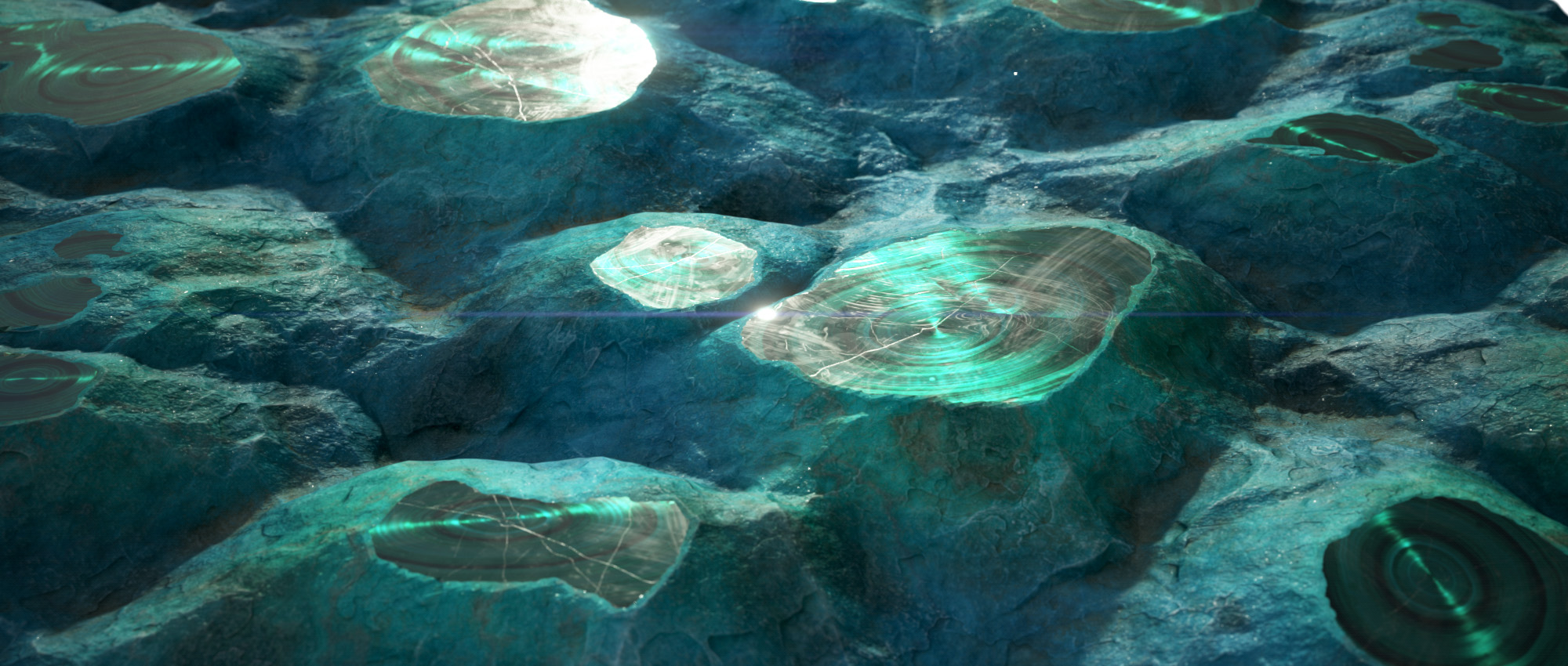
In this tutorial, I’m going to guide you through the creation of my Malachite with Chrysocolla Materialize competition entry. I’m going to cover the graph and MDL in full and then finally go into some detail on how I set up my final renders.
Preparation
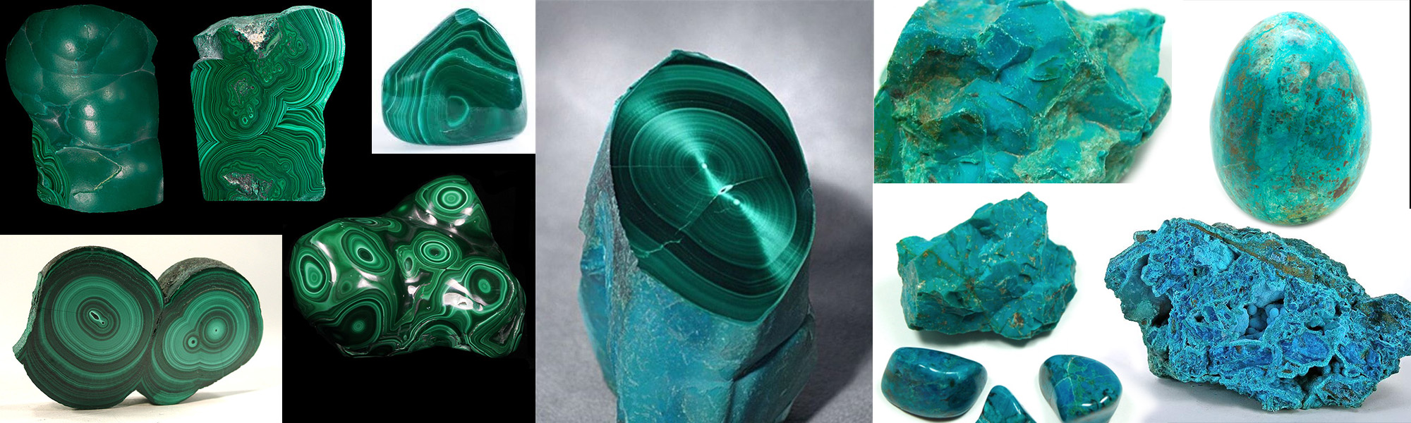
Before I even put my first node down, I had to decide whether I was going to try and recreate the reference image as precisely as possible, producing an isolated piece of malachite on a white background, or if I’d use the reference as inspiration to create a piece that recreated what I saw as the essential features in the reference, but filled in the blanks around the reference to become what was more of a traditional material. Ultimately I felt it made more sense to embrace the strengths of Substance Designer and translate as much of what I could see in the reference image into a procedural tiling material.
Having settled on an approach, my next port of call was to expand my reference library and to learn a little more about malachite. I started by gathering some extra reference images of other cut malachite samples. As well as the apparent malachite from the cut face of the reference, there is also the chrysocolla mineral coating on the outside of the malachite. So as well as malachite images I also gathered some other references of uncut stones showing off the chrysocolla coating on the exterior.
With a small collection of references gathered it was time to begin the creation of my material.
A Word on Optimization
But before we begin properly, I thought it would be useful to share a couple of tips that can help keep your graph running a bit faster.
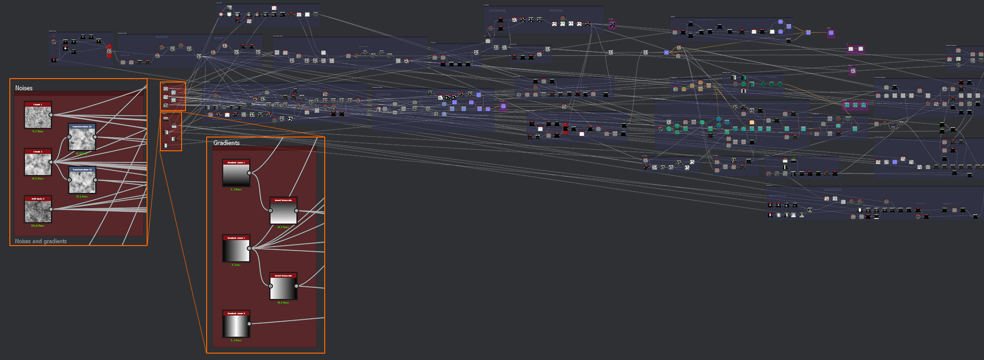
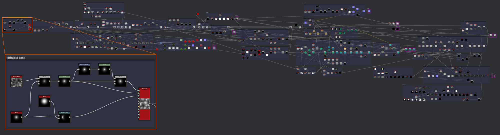
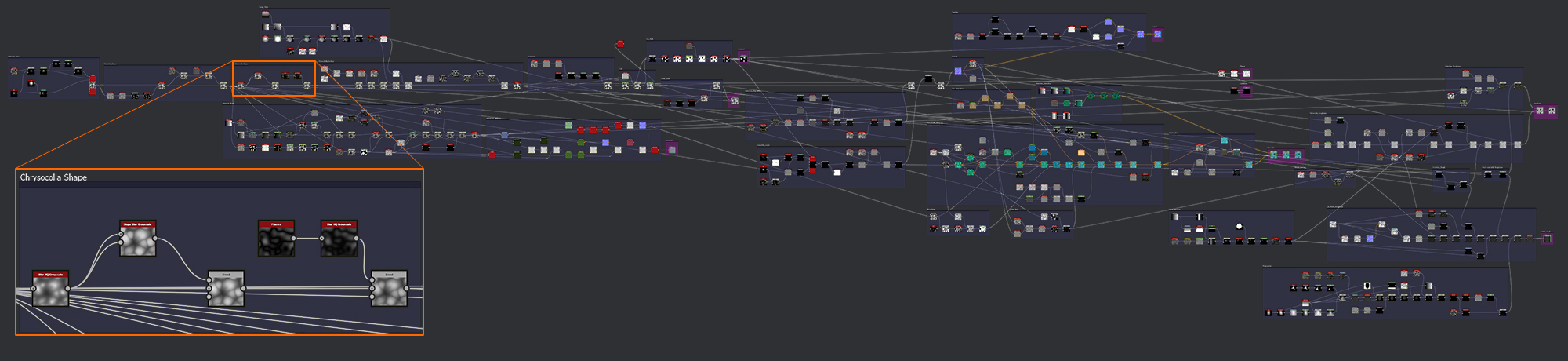
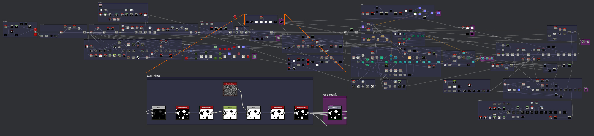
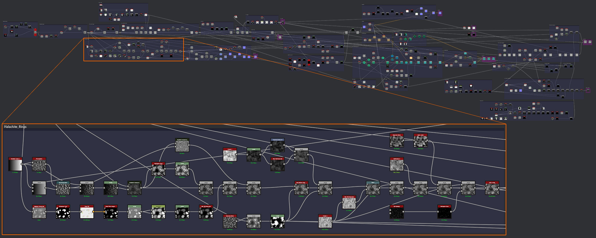
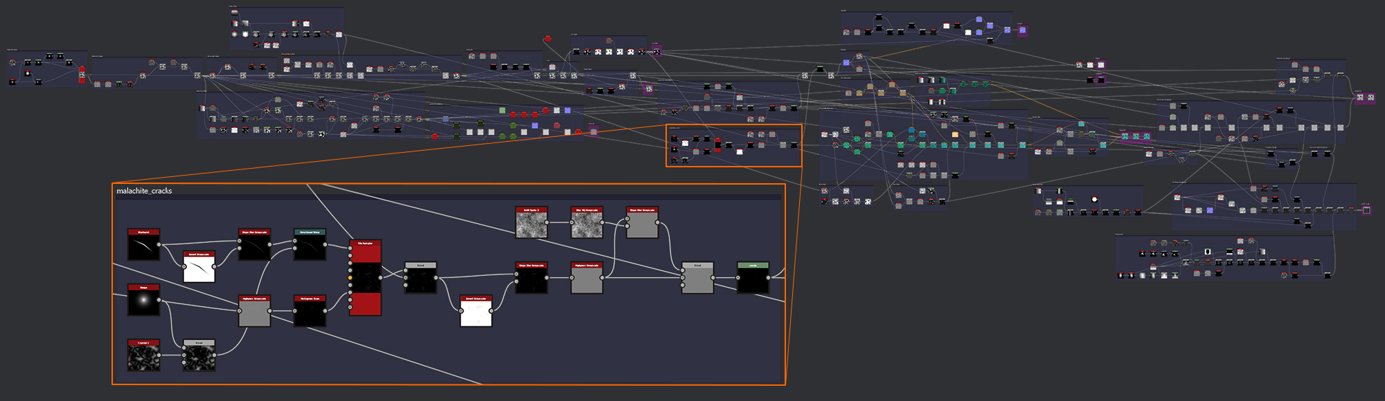
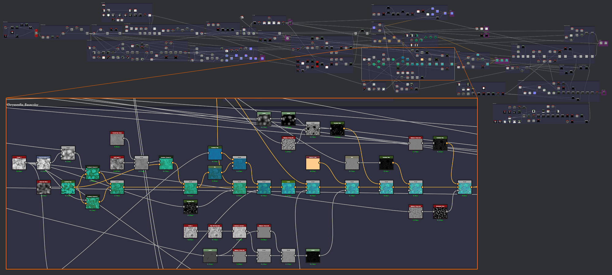
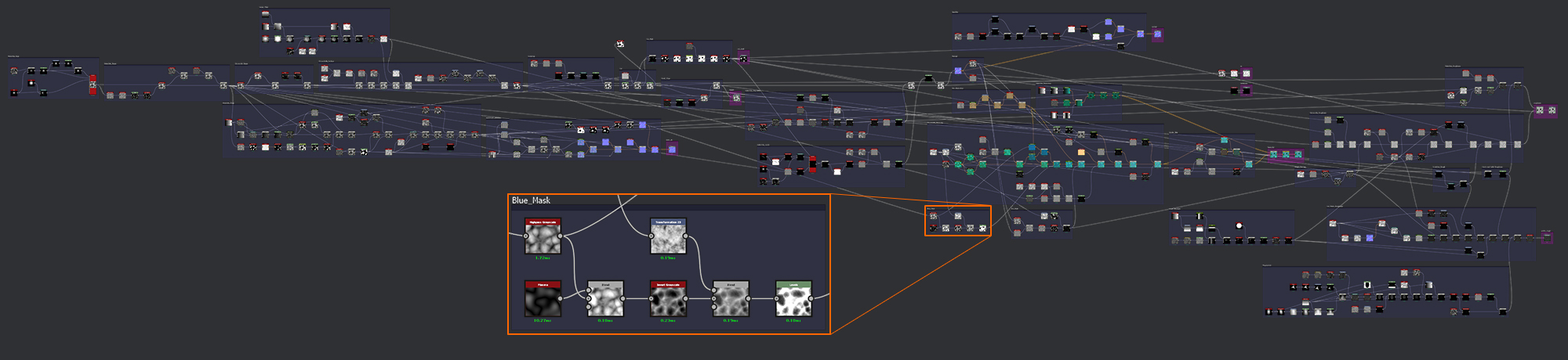
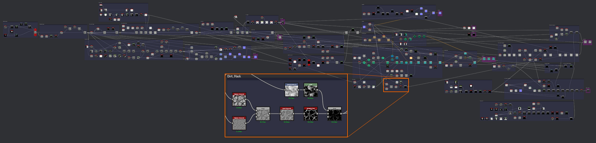
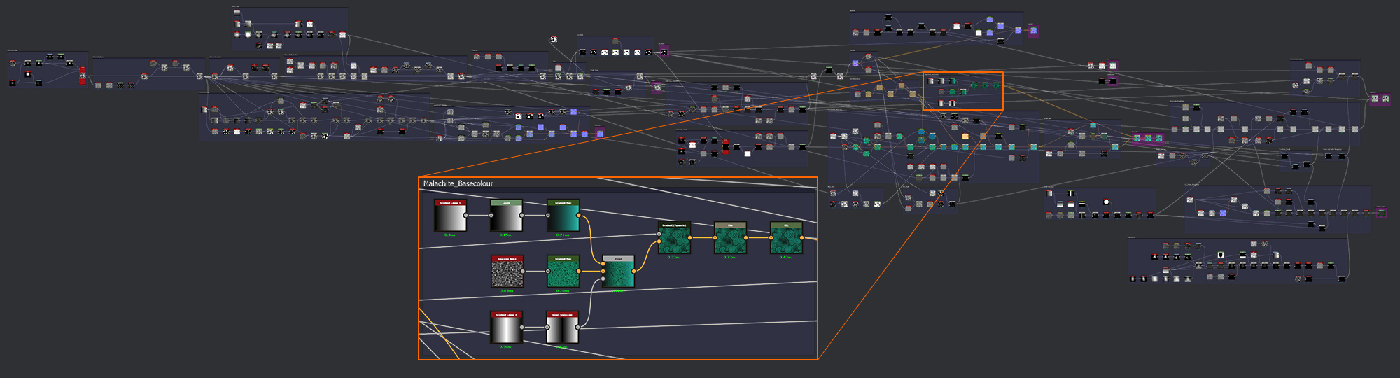
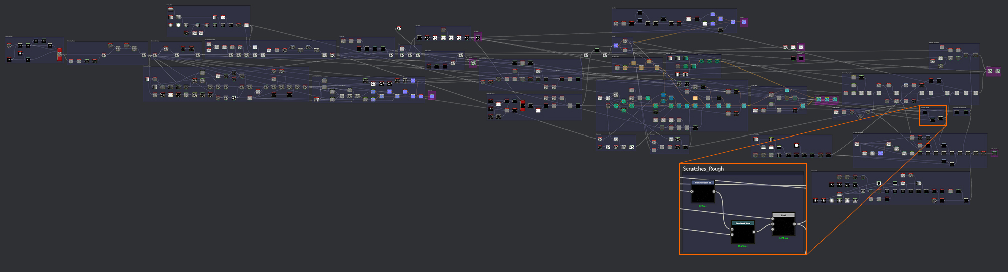
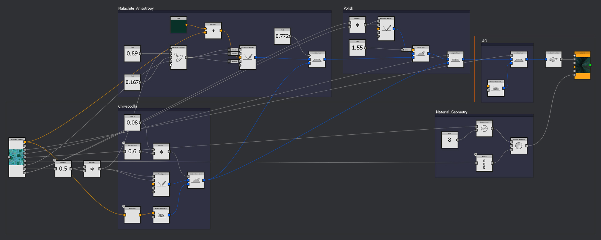
Node Reuse: Try to reuse as many nodes as possible rather than adding duplicates, as each duplicate node must be processed separately by the renderer. For this tutorial, I wanted to keep as many of the utilized nodes visible in each illustration as possible. So I chose to forgo this simple optimization for the sake of clarity. It also reduced the number of strands criss-crossing around the graph as they find their way to the shared nodes. As you can see here, the version of my graph that I submitted for the Materialize Contest reused a number of the generic input noises and gradients.
Node Output Size
: Another useful trick for speeding up your graph is to make use of the Output Size of individual nodes to reduce their scale relative to the rest of the graph. This is especially useful when you are creating inputs for a Tile Random node or Splatter node which take an input pattern. Often the resulting individual instances of the scattered input pattern will be smaller than the overall resolution of the graph. Therefore, you can reduce the scale of the input nodes to gain a few ms of render time. Another situation where this trick is useful is when using an input noise that may be blurred for any reason, such as the slope input to a Slope Blur Grayscale node. Reducing the resolution of the input noise can sometimes even negate the need for a blur.
You can see here that the resulting difference between the two outputs is extremely subtle. However, the first method using node scale clocks in at roughly 50ms, while the second approach takes nearly 80ms. The difference may be small, but it can add up to quite a processing time saving over a graph containing hundreds of nodes.
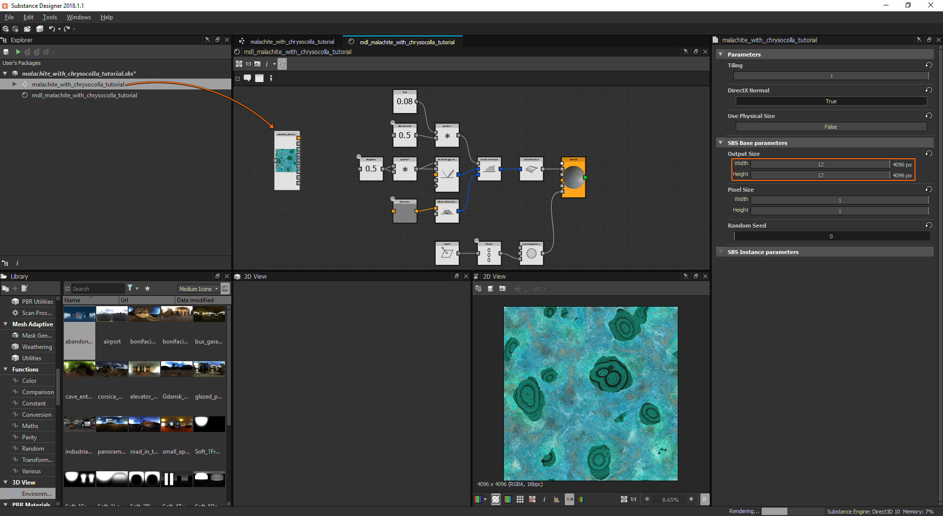
Graph Setup
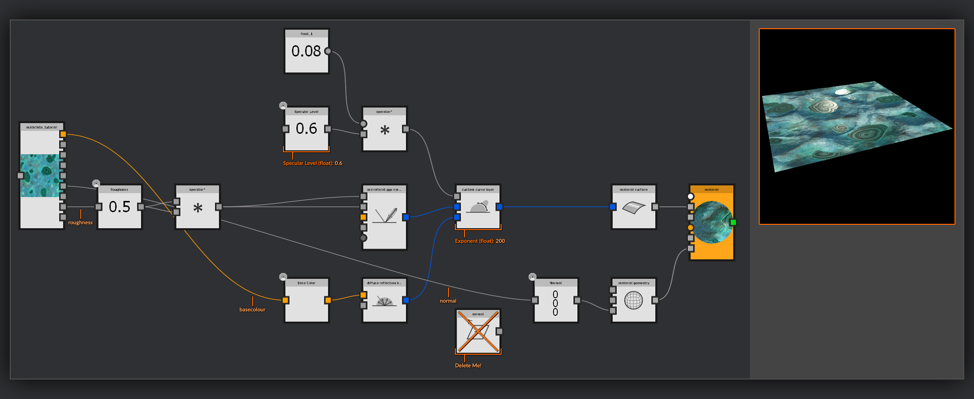
With some research done it’s time to get stuck in to building the material. First I’ll create a new Substance graph. I do this, and name it malachite_with_chrysocolla_tutorial. I choose the Physically Based (metallic/Roughness) template to give me some starting output nodes. For the size mode, I choose Relative to Parent and set the width and height to 2048. Working in 2048x2048 keeps everything running smoothly with quick updates to changes in the graph. As I plan on outputting the final material in 4096, I will however periodically check my adjustments in 4096x4096 to make sure I like what I see at that resolution. Finally, I set the format to 16 bits per channel.
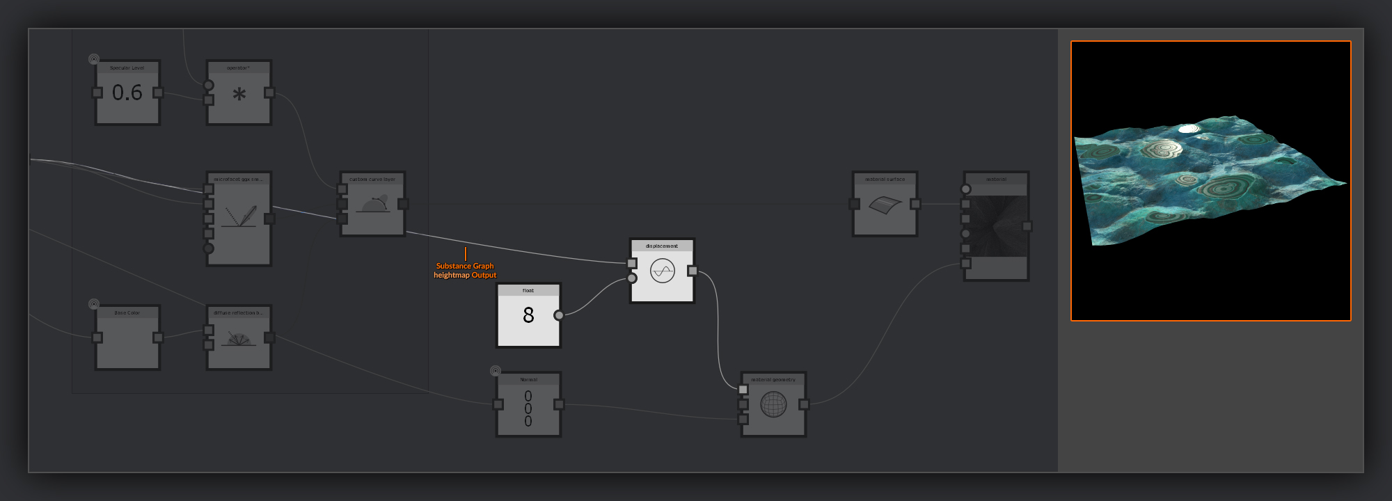
Heightmap
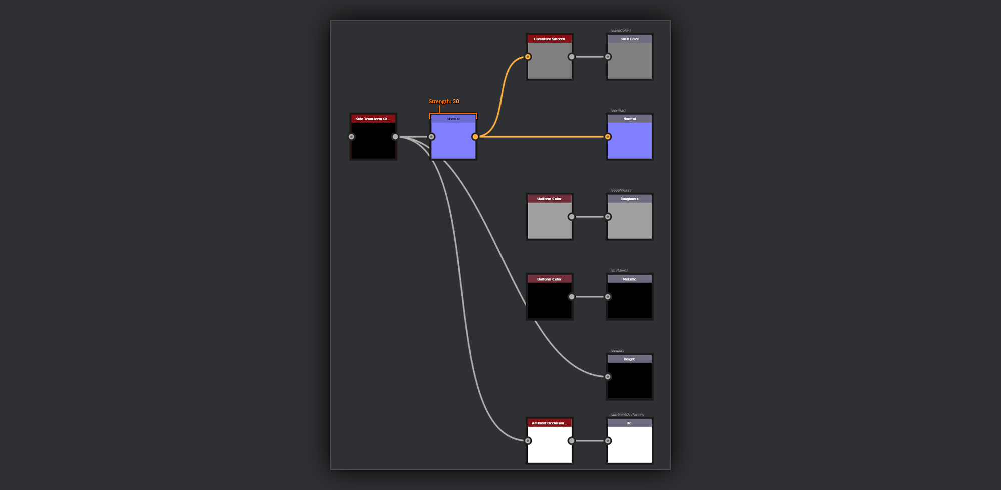
In nearly every material I create, I always begin by building up the Heightmap. For me, this is the most important part of creating a material in Substance Designer, as nearly every other output map relies quite heavily on the information set up in the Heightmap. While working on my Heightmap, I keep my outputs simple. The very first node I create is a Safe Transform Grayscale; I’ll feed my Heightmap output into this node before splitting off to my outputs later. Having the output passed through a simple node like the Safe Transform Grayscale provides a useful separation between the output nodes and my WIP graph. I attach the output of this Safe Transform Grayscale to the Height output. Then I add a Normal node
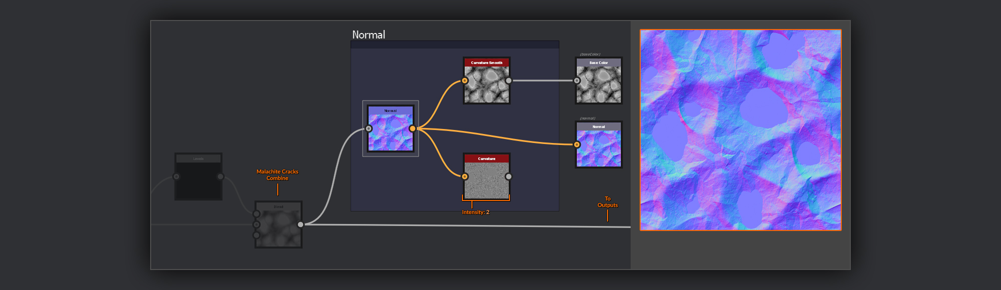
; for this piece I ended up with a relatively high Intensity of 30 in my Normal as I wanted to maximize the appearance of depth from the cut surface down to the valleys in the Chrysocolla. Usually, I finish around the 10-20 range, but in this piece, I found I was dealing with a lot of subtle noises over a fairly extreme Heightmap, so the extra boost to the Normal proved necessary.
I hook this Normal node output up to the Normal output node. From the Normal node, I also create a Curvature Smooth node and attach it to the Base Color output. The Curvature Smooth will help accentuate any edges or crevices I’m creating in my Heightmap. It also helps a lot to show how strong my noises are as I blend them in. For the Roughness output, I add a Uniform Color node set to slightly lighter than middle gray. I also add another Uniform Color node
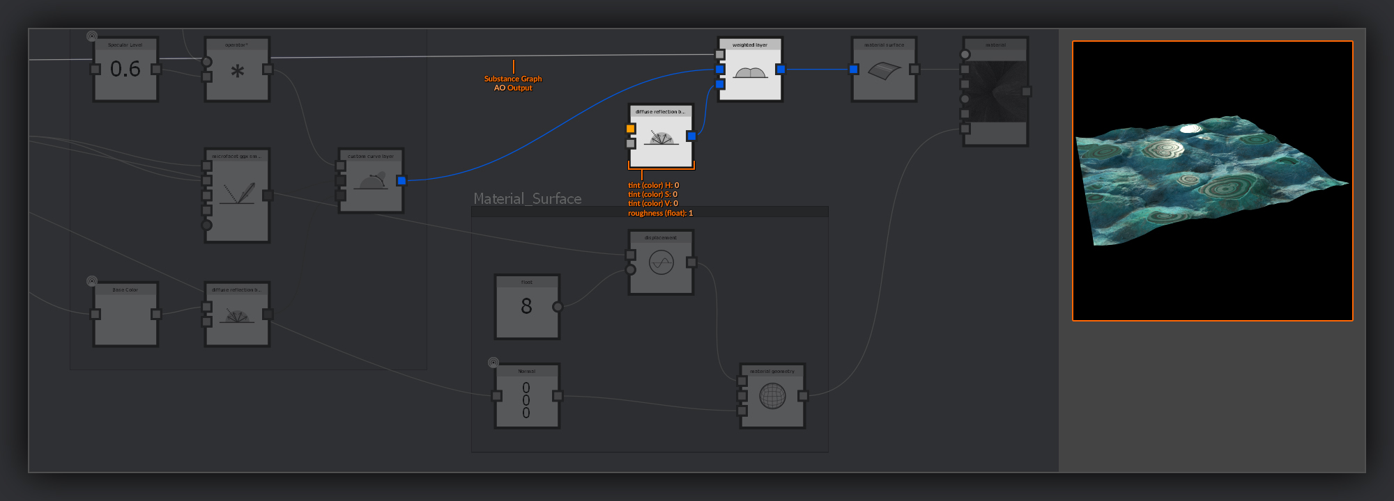
set to a black and attach it to the Metalness output node. For this piece, I’m going to use Ambient Occlusion separate from my diffuse, so I’ll create an Ambient Occlusion node and attach this to a new output node set to ambient occlusion in its usage. It’s important to label it accordingly. Keeping the outputs simple at this stage is going to help me stay focused on getting the precise details I want in my Heightmap before I move on to adding other information in the BaseColor and Roughness passes.
Malachite Base
Now, with my outputs set up, I’m ready to start working on the graph. I begin by building or growing the stone as organically as possible. In the reference, I’ve seen that the surface of a piece of unbroken malachite is often made up of some bubbly nodules, so these are what I’ll strive to recreate. The first step is to get the large shapes down. These are going to provide the peaks I will eventually cut away to reveal the malachite and the valleys where the uncut chrysocolla surface will remain.
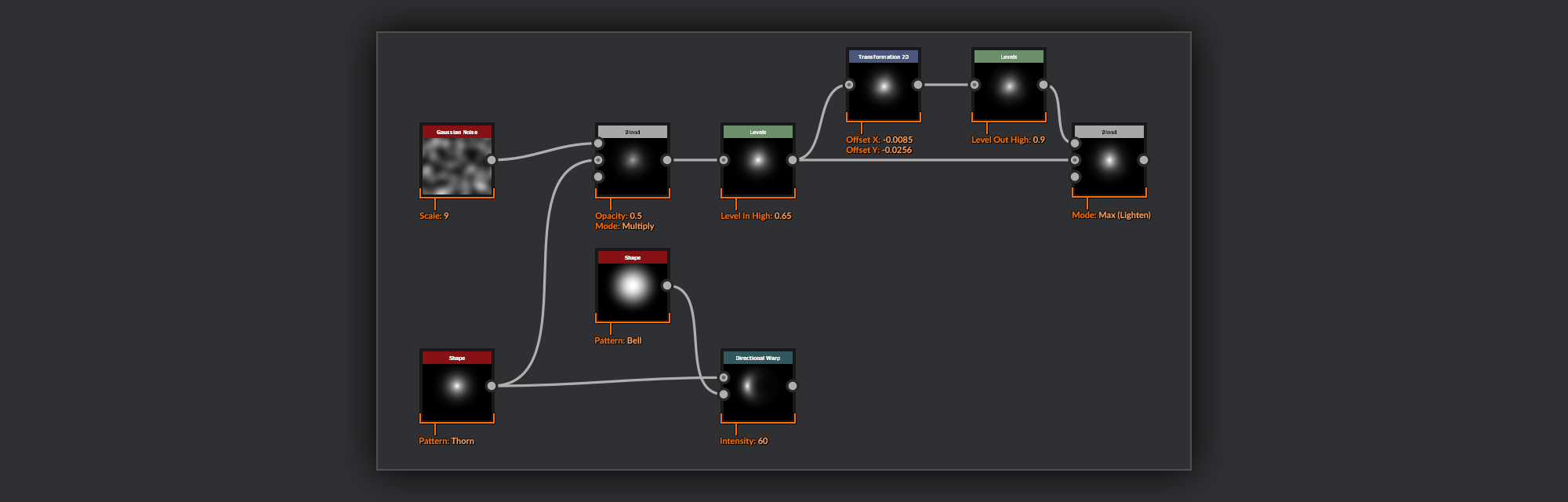
For the base of my malachite, I use a Shape node with the Thorn Pattern
. I chose this shape because the nonlinear gradient from the base to the point of the thorn means the output from the Tile Sampler will have a good contrast between the peaks and the valleys. This will prove super-useful for pulling some masks out for the rest of the graph, such as for creating the Normal map used by the anisotropy in the MDL. I started with two variants of this thorn shape, one slightly squashed and bent around a Shape node using the Bell Pattern with a Directional Warp node to produce some variation in my Malachite Surface. On the other thorn, I add some Gaussian Noise in a Blend node set to Multiply; this helps to break up the uniformity of the shape.
When working on this material for the contest, the result I was getting once these thorn shapes were scattered didn’t feature the satisfying combination of peaks as seen in the Mattershots reference Image, where two peaks are very close together. I chose to manually create this combination by combining two of my thorn shapes by hand.
I use a Transform 2D node to offset one Thorn from the other, and a Levels node to slightly drop the height of this new peak down slightly. Finally, I combine these two in a Blend node set to Max (Lighten).
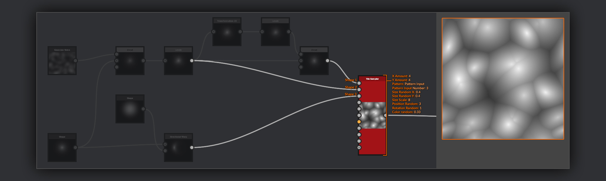
These three base thorn shapes are then used as pattern inputs of a Tile Sampler node
. I set up the Tile Sampler to scatter the shapes pretty evenly across the canvas with a little bit of clustering and some slight scale variation.
The last step here is to frame up the nodes we’ve made to keep the graph organized.
Malachite Shape
Now, having completed a very basic pass defining the shape and location of each nodule, I move on to refining the base shapes to create the final surface shape Heightmap upon which the rest of the graph will be built.
The first thing to do is smooth out the valleys between the nodule peaks; I want to make sure they are not too sharp, as that might impact the organic appearance.
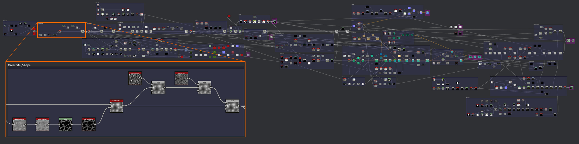
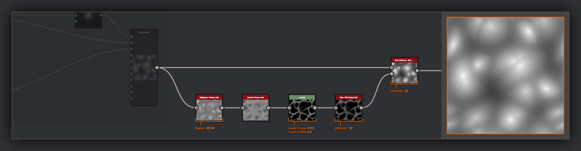
To do this, I’ll make a mask with which I can isolate the valleys, and then blur them to soften them. The first step is to create a mask that will isolate the valleys of the Heightmap output from the Malachite Base. I do this by taking the output of my Malachite Base and putting it through a Highpass Grayscale node to remove some of the height variations. I then Invert the output and pass it through a Levels node
where I clamp the Level in Low to isolate the valleys; I also bring the Levels In Mid down to make the falloff to black less harsh. This mask is then fed into a Non Uniform Blur node in the Blur Map input with my Malachite Base in the Grayscale Input.
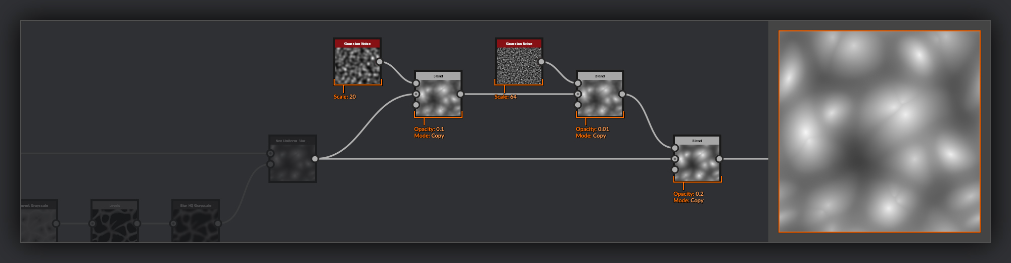
Next, I add a tiny amount of noise with a couple of Gaussian Noise nodes set to different scales. Each is combined with the Malachite Base using a Blend node set to Copy and a low opacity. This will prevent the malachite rings that I’ll add later from being perfectly concentric, helping them look more organic. I copy the noiseless output from the Non-Uniform Blur back over this noisy version with a Blend node
set to Copy in order to control more precisely the strength of these combined noise passes.
At this point, the graph diverges between the sections used for the cut malachite surface, and what will become the outer chrysocolla layer. So I’ll frame up the nodes added to the Malachite Shape before moving on to the Chrysocolla which I’m going to focus on first.
Chrysocolla Shape
After the divergence, I’ll begin making adjustments to the Heightmap that will be the beginnings of my Chrysocolla Shape. I’ll start by creating the more pillowy appearance of the raw malachite, over which the chrysocolla will have grown.
First I’ll increase the volume of the malachite nodules - I want a more bulbous surface for my malachite, as opposed to the spiky surface the raw Thorns output will currently provide.
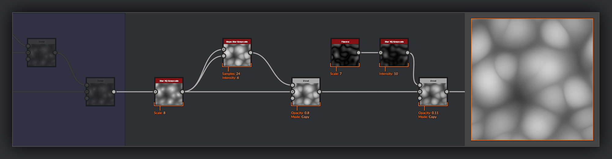
I start by blurring the output of my Malachite Shape in a Blur HQ Grayscale node, I then use a Slope Blur Grayscale node
with the output of the Blur HQ Grayscale in both inputs to inflate the thorn shapes. Finally, I add in a small amount of Plasma node noise, softened with a Blur HQ grayscale, this is combined with the Chrysocolla shape using a Blend node set to Copy with a low opacity. This plasma noise is going to add some medium surface variation before adding finer detail in the following stages.
With the main shapes taken care of, it's now time to start refining and detailing the surface of my Chrysocolla Heightmap. Be sure to frame this section up before moving to the next.
Chrysocolla Surface
I’m going to add my surface detail using a few different layers of noises with both smaller and larger scales.
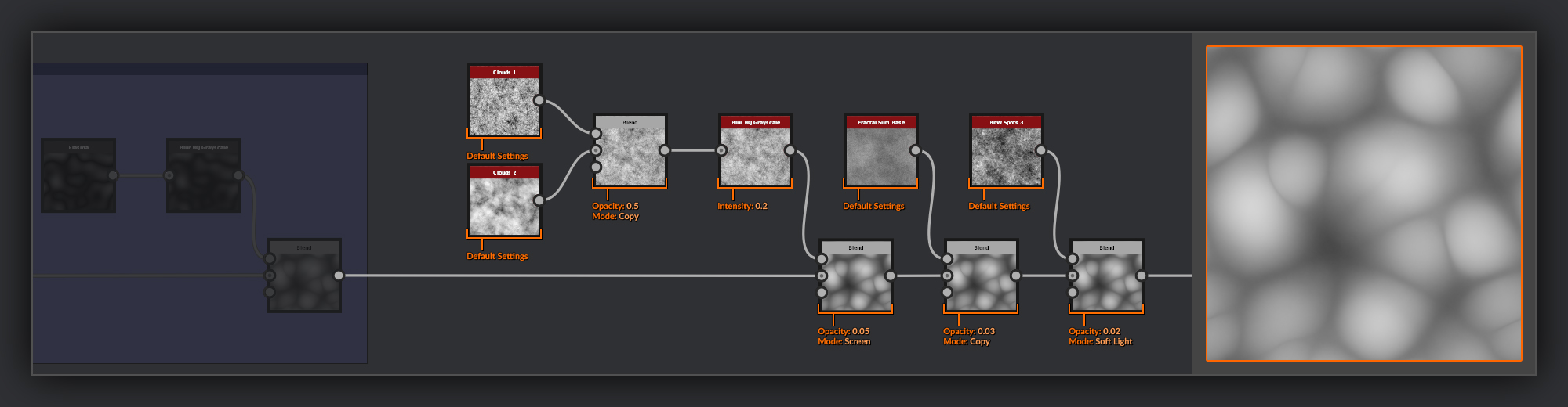
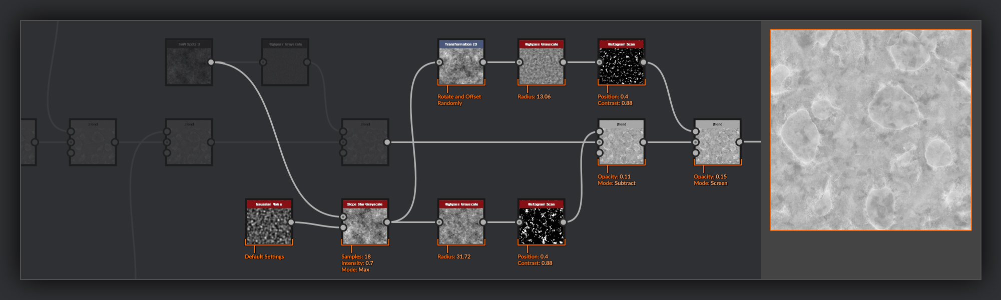
The very first layer of detail I blend in is some noise made by combing a Clouds 1 node with a Clouds 2 node 50/50 using a Blend node set to Copy. I like to do this as it mixes up the detail frequency nicely and also reduces contrast in the noise somewhat as a convenient byproduct. I then very slightly soften this in a Blur HQ Grayscale node to remove the highest frequency detail before adding this over the previous Malachite Shape Heightmap with a Blend node
set to screen and a very low opacity.
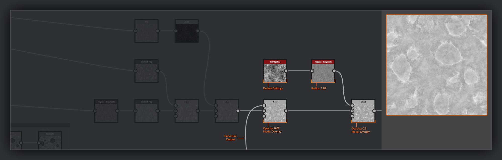
Next, to get a gritty feeling to the surface, I blend over a Fractal Sum Base node. I use a Blend node set to Copy, again with a very low opacity. I follow this by a BnW Spots 3 node which I add using a Blend node set to soft light to add some medium-scale information to the grittiness.
Now I want to focus on giving the surface a rocky appearance. So in the next pass, I’ll add some medium to large shapes that will make the surface look more like it has been dug out of the ground.
Large Chips
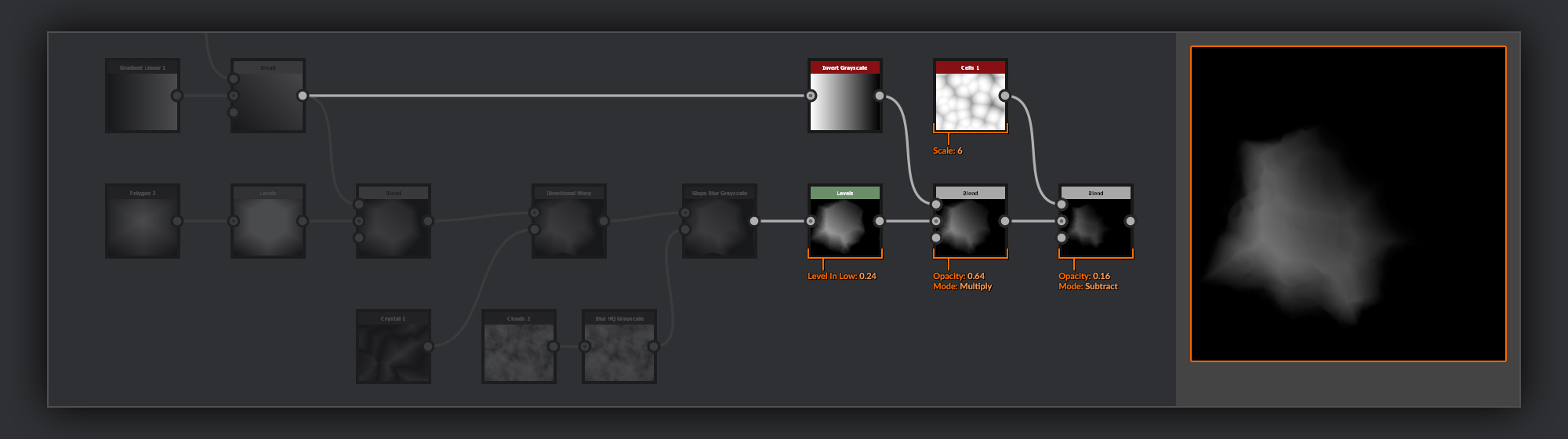
First up, so the piece doesn't end up looking too pristine, I will be adding some chips that have been taken out of the surface of the chrysocolla. This slightly more angular detail will also contrast well with the softer organic shapes we currently have in the chrysocolla Heightmap.
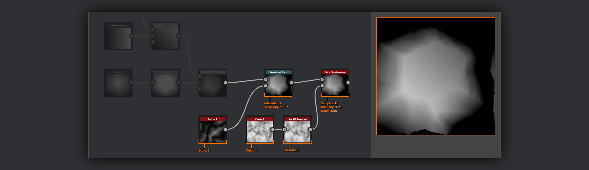
I start the large chips with a Polygon 2 node. I’ve set it to 6 sides and increased the scale to 1.5 to give me plenty of range to play with when it comes to mixing up and eroding the shape. I begin sculpting my individual chip shape by flattening out the top of the polygon with a Levels node. Next, I combine 2 Gradient Linear 1 nodes
evenly at 90-degree angles to each other in a Blend node set to Copy; this gives me a diagonal gradient. I combine this with a Blend node set to subtract which provides me with an overall slope in the volume of the chip shape.
The next thing I do is add some angels to break up the silhouette of the chip, I do this with a Directional Warp node using a Crystal 2 node as the Intensity input. After this, I use a Slope Blur Grayscale node
to add some micro surface chips to my large chip shape. The Slope Blur Grayscale has its mode set to Min, which means only resulting values below the input values will show in the output. This is super-useful for adding chips or other subtractive surface damage. For the slope input, I use a Clouds 2 softened in a Blur HQ Grayscale node.
Then I use a Levels node to bring up the Levels in Low, making sure the whole of my chip shape is contained within the canvas and not spilling outside. I accentuate the slope one last time by taking an inverted copy of my 90 degree rotated Gradient Linear 1 and multiplied it over my chip height in a Blend node
with middling opacity. Lastly, I add some overall surface undulations to the chip shape by subtracting a Cells 1 node from the chip shape below.
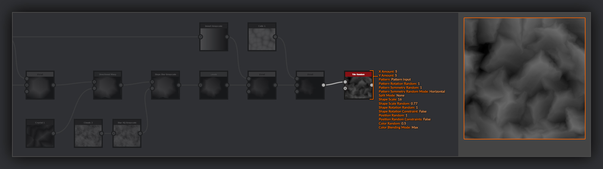
The chip shape is then scattered using a Tile Random node. Here, I was looking for an even distribution of gray values; I didn’t want any peaks or valleys that were too strong. I also wanted a nice mix of scales, with some flatter areas with larger individual chips as well as other noisier areas with more chips clustered together.
Finally, I’ll frame these nodes up as they exist somewhat independently from the main Chrysocolla Surface chain.
Back to Chrysocolla Surface
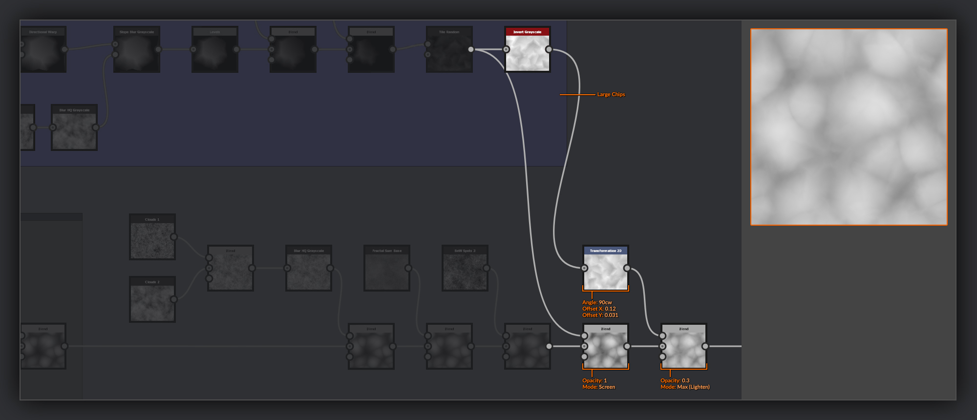
Going back to the Chrysocolla Surface, I’ll mix this Tile Random output into the Chrysocolla Heightmap.
I combine the first pass of the chips by adding them over my Chrysocolla surface Heightmap in a Blend node set to Screen. This is going to help add some sharper rocky shapes to the Heightmap. On the next pass I invert the chips after the output from the Tile Sampler with an Invert node. I then shift the chips around the canvas slightly using a Transform 2D
to mix up their translation and rotation to ensure they cover different areas of the surface to the previous layer. This transformed copy is then combined with my Chrysocolla Surface using a Blend node set to Max Lighten, so it only adds a few rocky peaks here and there in between the peaks on the Chrysocolla surface. I lower the opacity to make sure they don’t end up standing too proud of the surface; I don’t want them interrupting my cut surfaces too much.
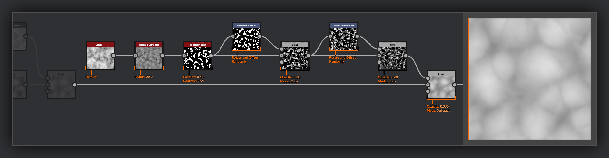
After the larger rocky shapes, I want to add some sunken patches where the outer layers of chrysocolla have flaked off.
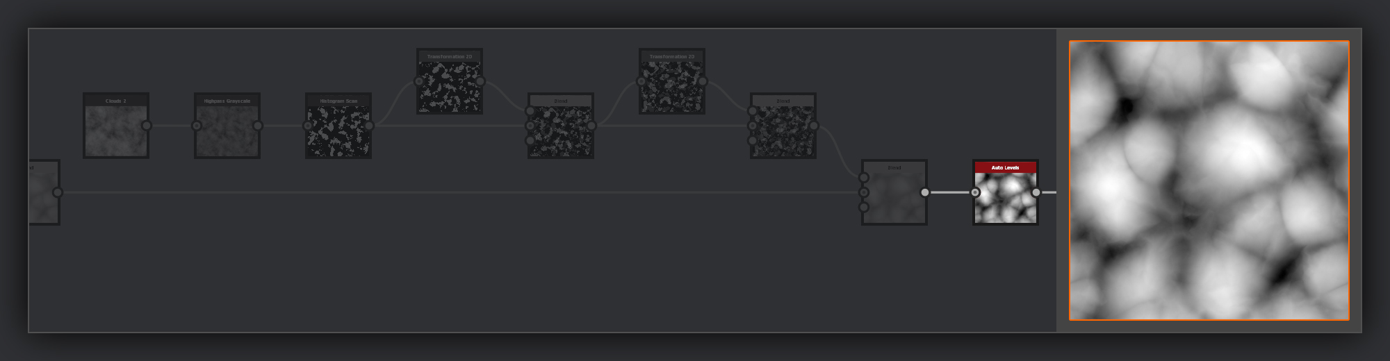
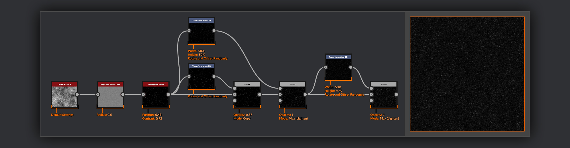
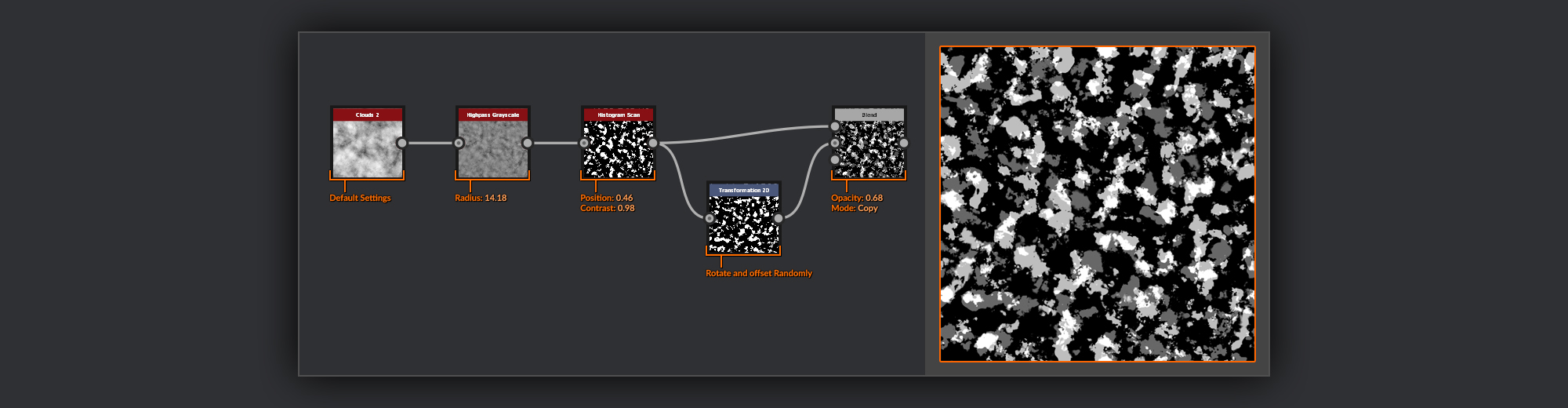
For these, I’ll start with a Clouds 2 node
and even out its range using a Highpass Grayscale node. Then with a Histogram Scan node, I select a slice of noise from the clouds. Next, I use a Transform 2D to rotate and offset this slice, before adding it over the previous slice in a Blend node set to Copy. I repeat this process again with the now combined slices to add a further layer of patches. Finally, I combine this with my Chrysocolla Surface in a Blend node set to Subtract to sink these patches into my Heightmap subtly.
Finally, I add an Auto Levels node
to make sure I’ve got the full range of black and white to work with. This is important in this graph because I want to use this Heightmap to create the division between the outer chrysocolla and the malachite inside. Usually, I try to avoid relying on the Auto Levels node as it slows graphs down somewhat, and can generally be avoided by managing your levels carefully in other places. Here, however, having a full range of values to work with makes the following steps more predictable.
As this is the end of the Chrysocolla Surface, I’ll also frame these nodes together now.
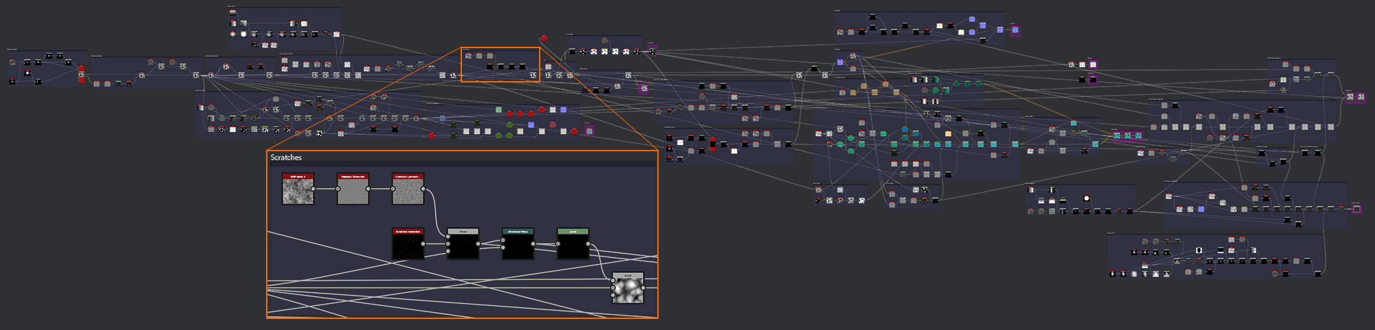
Scratches
The final detail I want to add into the Heightmap for my Chrysocolla surface is some fine scratches. Subtle scratches help with achieving some realism, by giving it the look of something that hasn’t been kept pristine.
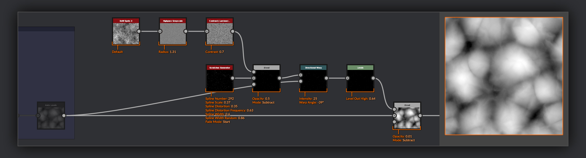
I use the Scratches Generator node to create the scratches. I then break the scratches up a bit using a BnW Spots 3 node passed through a Highpass Grayscale node with a low radius. I combine this with the scratches using a Blend node set to Subtract. Next, I warp the resulting scratches over the Chrysocolla Heightmap with a Directional Warp node. This helps ground them on the surface. The last thing I do is add a Levels node
to bring down the Levels out High before proceeding to combine them with the Heightmap below in a Blend node set to subtract. Using the Levels node helps to control the subtlety of the scratches when coupled with the opacity strength of the Blend node.
The scratches are the last detail needed for the chrysocolla surface. From now on we’ll be dealing with the cut malachite. I finish the scratches section by framing the nodes together.
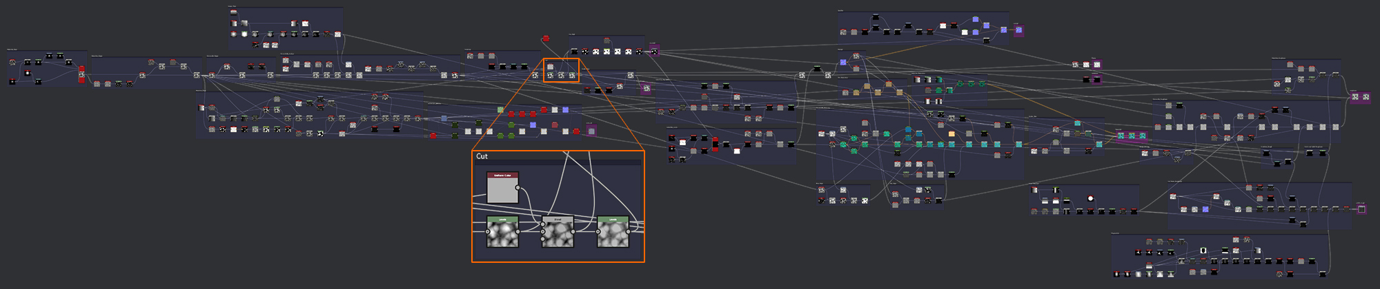
Cut
Now it’s time to perform the slice that will give us the cut faces on the surface of the material and reveal the malachite below the chrysocolla.
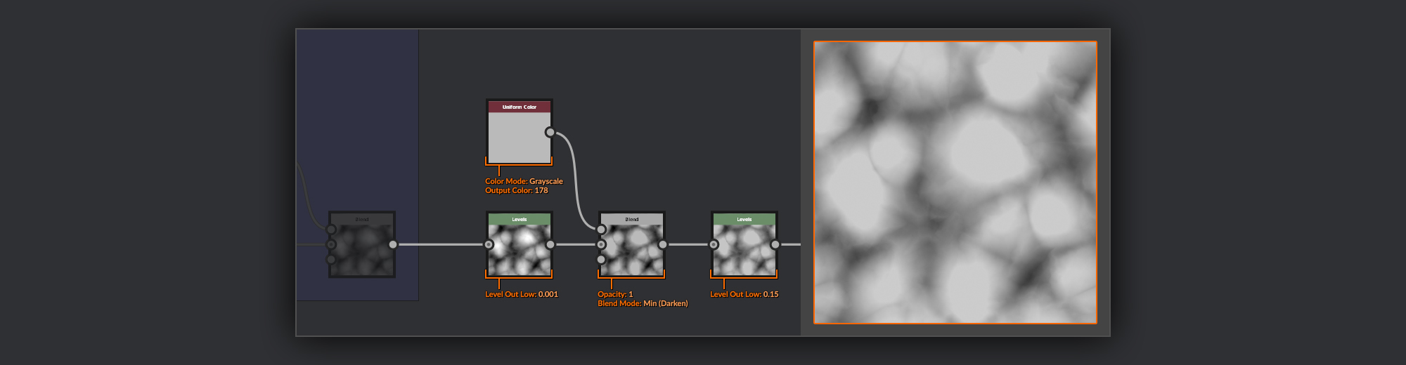
I begin again by adding a Levels node and bringing the Level Out Low up by a tiny amount; this ensures I haven’t already hit black anywhere in the Heightmap before processing it for the cut. I follow this with the cut itself, which is pretty straightforward. I use a Uniform Color node with a gray value to define the depth of my cut. I combine this gray value with the Chrysocolla Shape Heightmap in a Blend node, using Min (Darken) as the blend mode. After the cut, I also add a Levels node
and raise the Level Out Low slightly. I need to ensure that even if I use a cut level of 0 the Heightmap is never going to end up with a height of zero; this will ensure there will always be some gray value to subtract from in the next steps.
Any value in the Heightmap above the value of the gray in the Uniform Color node will be flattened down to match the value of the Uniform Color, providing a smooth flat surface to take for the cut malachite.
Here I frame up the nodes that make up the cut step and move on to creating a mask for the cuts themselves.
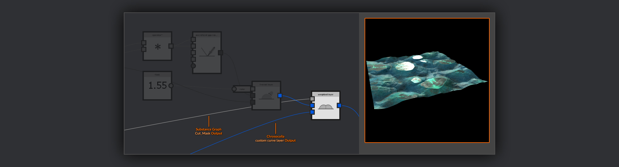
Cut Mask
Now I have this flat surface where the cut has been made; I need to pull that specific range out from the Heightmap to turn into a mask which I’ll use to split my graph between the two materials.
To isolate the cut surfaces, I’ll find the difference between the original surface and the new cut surface.
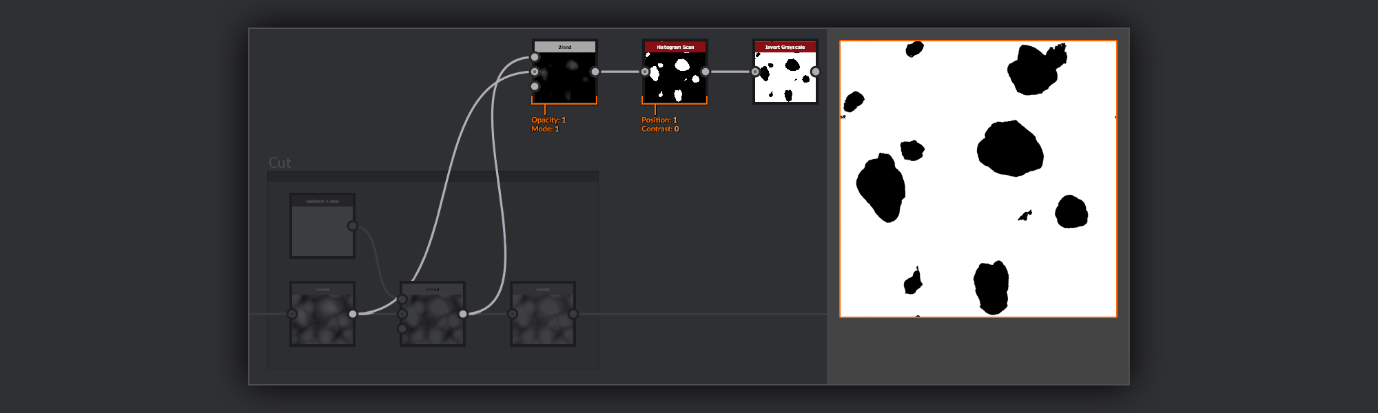
I do this using a Blend node
; I place the resulting cut Heightmap, from after the Blend node, into the foreground; in the background I place the pre-cut surface from the output of the Levels node. I set the blend mode to Subtract; this will cancel out any values that are the same as or darker than the background input, in this case leaving only the peaks above the cut surface. I can then use a Histogram Scan node to isolate the peaks to give me the top layer of pixels of each cut surface. Finally, I use an Invert node so that the cut faces themselves are white.
Once the basic mask is done, I want to add some nodes through which I will add some thickness to the chrysocolla surface surrounding the malachite.
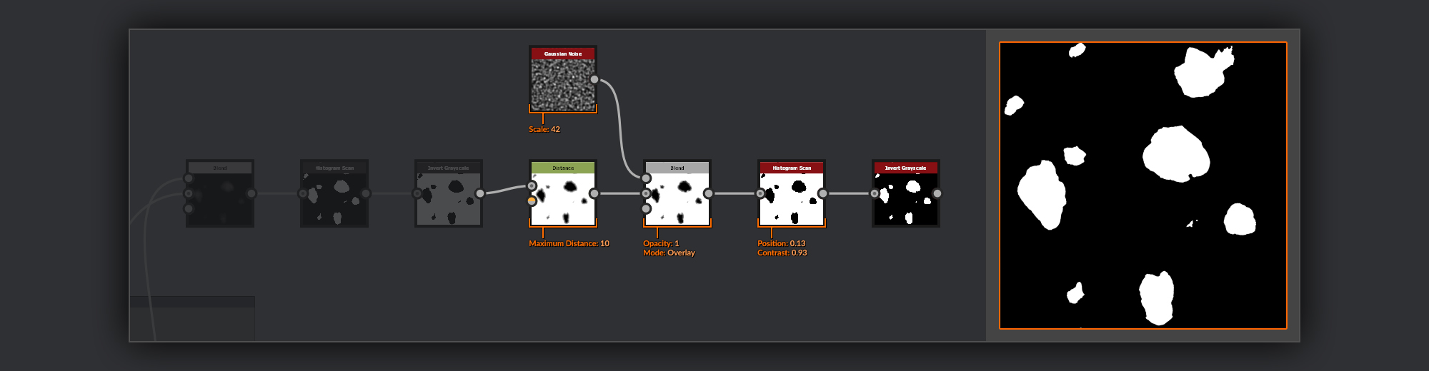
I pass my mask through a Distance node to create a gradient border around the cut sections. I then combine this with a Gaussian Noise node in a Blend node set to overlay. This is going to vary the values in the gradient border around the perimeter of the cuts. To get the final malachite regions, I use a Histogram Scan node to create a new slice from this height information.
The final step here is to again invert the mask so that the cut sections are white in the mask.
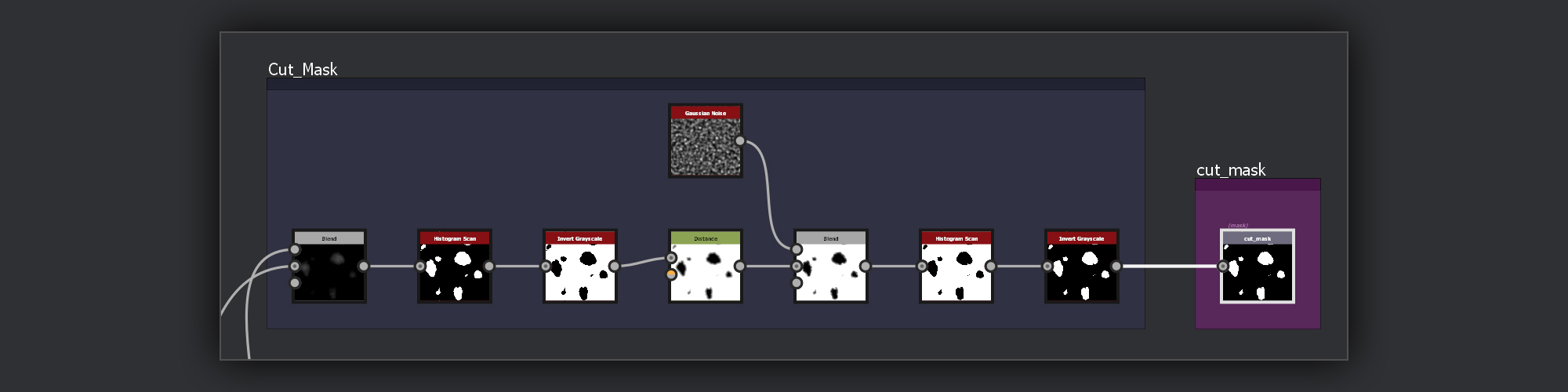
As with finishing the past sections, I now frame up the cut mask. This time, however, I also add an Output node, and I give it a label of cut_mask to make it recognizable. I also like to frame my outputs separately in a brighter color than the default, which I usually stick to for all outputs; this helps them stand out later on if I want to revisit them for any reason.
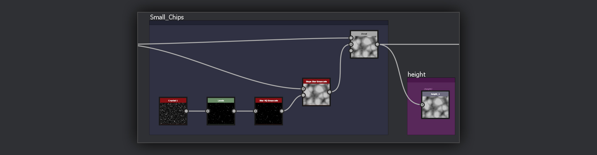
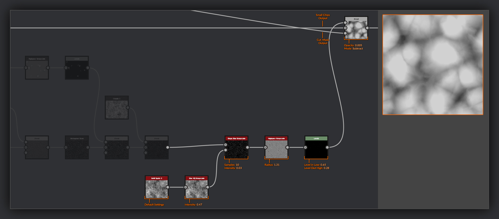
Small Chips
With the cut surface added in, there is only one final detail I want to add to my Heightmap. Some smaller chips to the surface that will also be removed from around the edges of the cut surfaces.
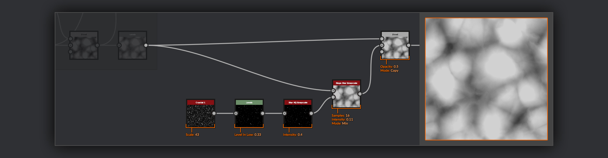
To make my small chips I’ll take a Crystal 1 node with a small scale. Then using a Levels node I bring the Level In Low up until I have just a few peaks of the Crystals left. I soften this with a Blur HQ Grayscale node. I feed these isolated peaks into the slope input of a Slope Blur Grayscale node with my Malachite Heightmap fed into the Heightmap. I use a blend mode of Min with a low Intensity to slightly erode the surface of my Malachite. Finally, I combine this with an unchipped copy of the Heightmap in a Blend node to reduce the strength of the chips slightly.
At this point, the small chips get a frame of their own, and as the Heightmap is complete, I’ll move my output node for the Heightmap to the end of this frame. I leave the other outputs behind the Safe Transform Grayscale for now.
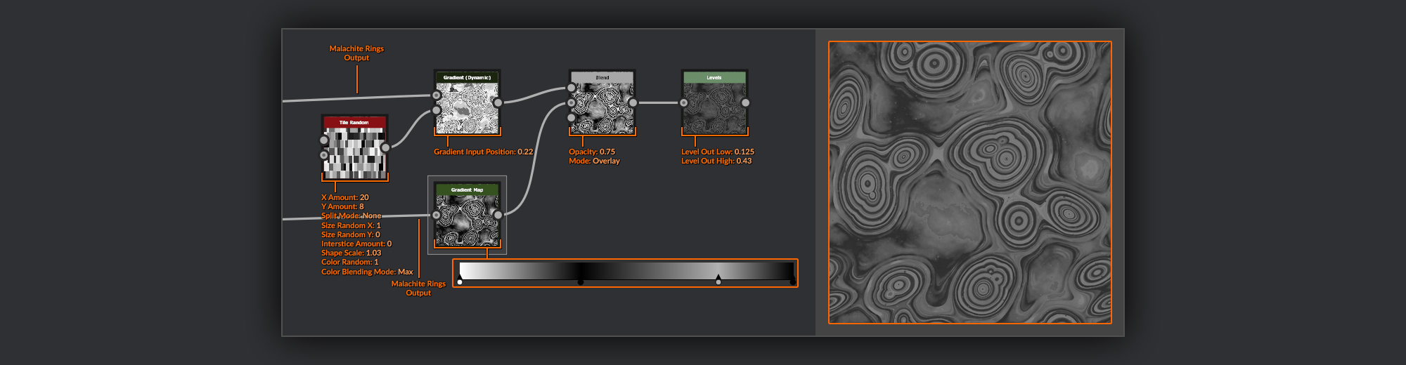
Malachite Rings
Now It’s time to start working on the node string that will form the surface of the cut Malachite. The first part of this is to create some grayscale maps that have all the various rings visible on the surface of the malachite.
First I create a palette of sorts, from which the gradients of my rings will be selected.
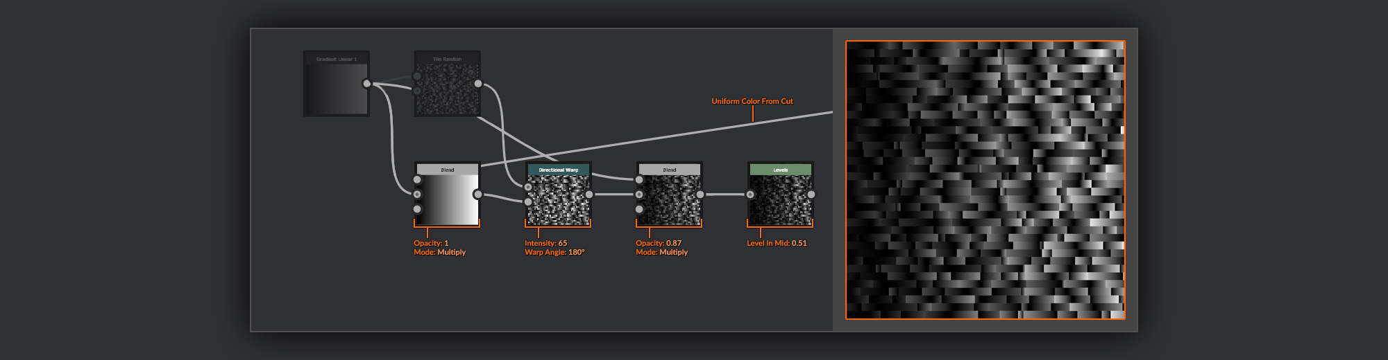
For this, I create a Tile Random node with a Gradient Linear 1 as the input. I mix up the scales, directions, and luminosity of the resulting gradient tiles.
I like to create palettes to pull values from for Gradient Dynamic nodes, rather than using plain Gradient nodes as it allows you to modify the gradient in various ways beyond simply creating a new gradient. It also gives you the option to select different input regions of a palette in the Gradient Dynamic node which can be more useful than rearranging the pins in a regular gradient.
Later on, when I was rendering my original contest entry, I realized that I wanted to have the rings change in the way you might expect as the depth of the cut was increased.
To do this here, I just combine the output of the Uniform Color that defines my cut depth with the Gradient Linear 1 in a Blend node set to multiply. I then use this as the Intensity Input for a Directional Warp node with the Rings Palette as the Input. Now when the cut level is shallow, the rings will be more stretched out and therefore broader than when the cut is deep. After making my adjustments for the cut depth variance, I combine the output of the Tile Random with the Gradient Linear 1 in a Blend node using Multiply. This means I will still have a rough High to Low transition across the width of the output rings. Finally, with a Levels node, I increase the Level In Mid a little to bend the gradients slightly away from a linear gradient, which helps to give them a bit more body.
Here’s an example of the rings being stretched as the cut height is adjusted.
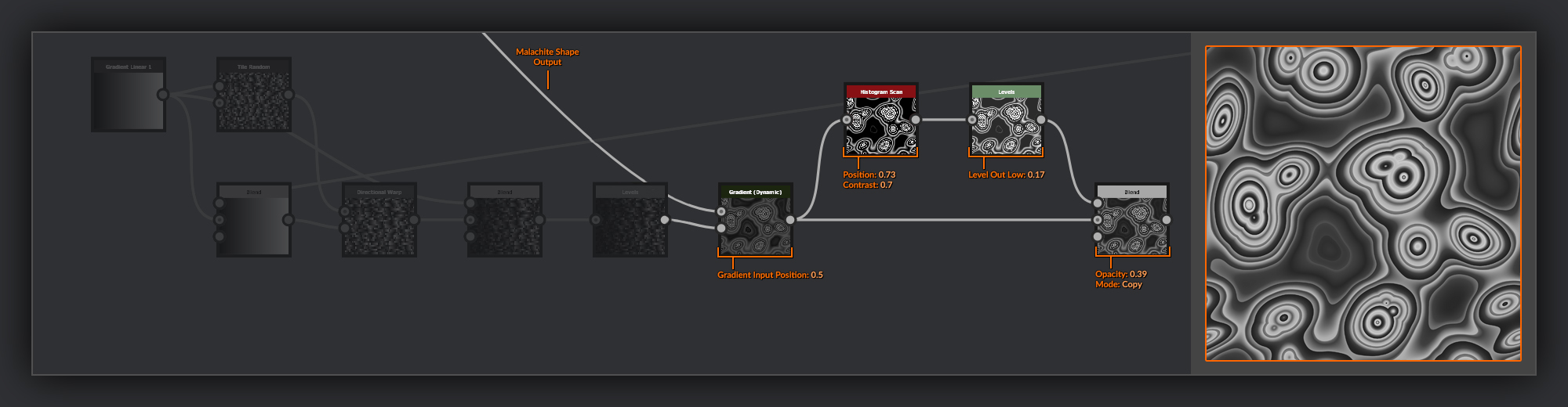
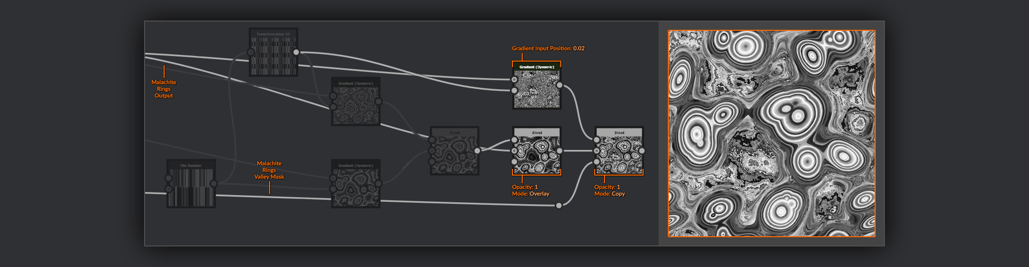
Now I can use this palette to add rings to my malachite Heightmap.
I take the output of the Malachite Shape and pass it into the Heightmap of a Gradient (Dynamic) node using my Gradient palette previously as the gradient input. After this, to embolden some of the rings further, I’ll take the output of this Gradient (Dynamic) node and run it through a
Histogram Scan to increase the brightness of the gradient peaks. With a Levels node, I then bring the output low up slightly before copying it back over the Gradient (Dynamic) output in a Blend node with medium opacity.
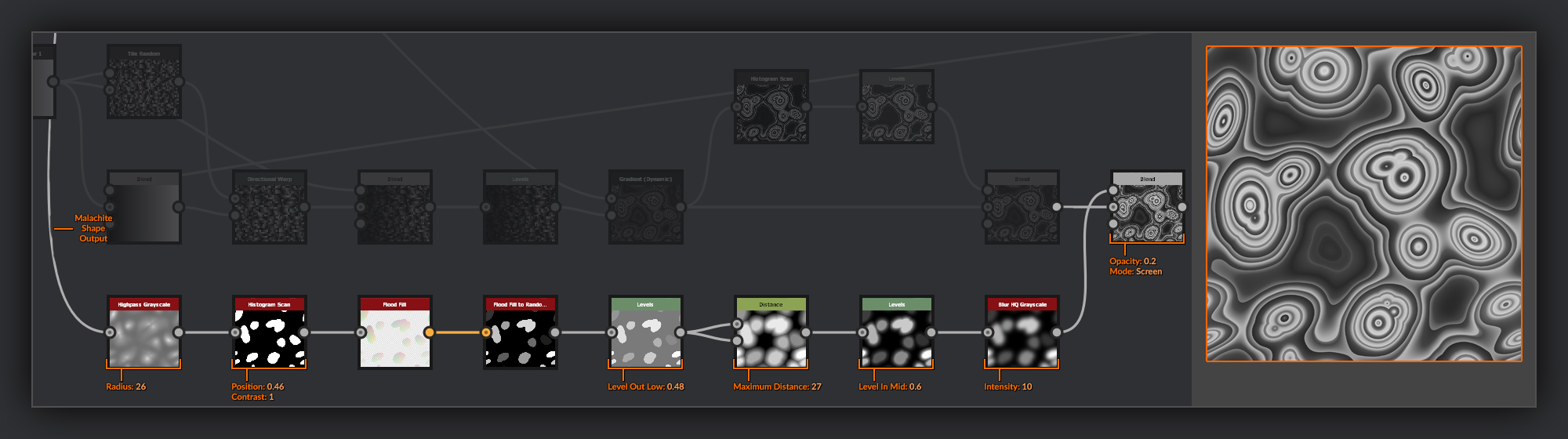
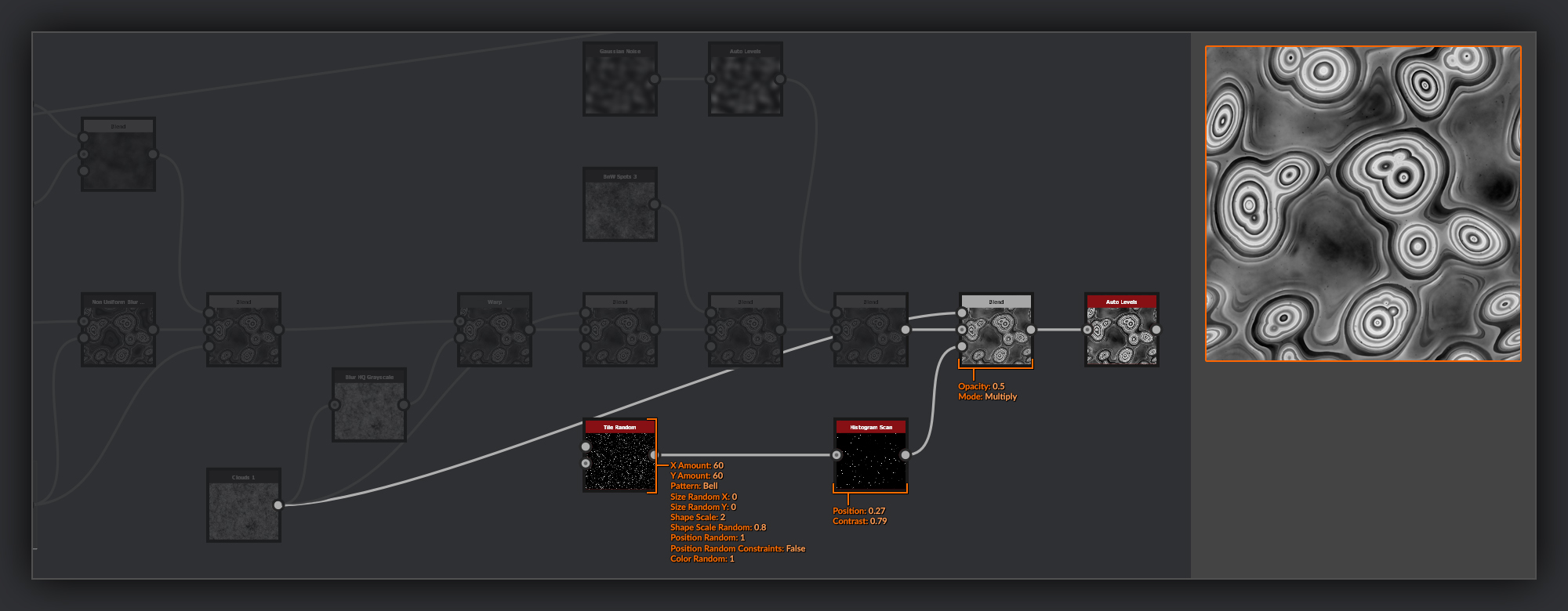
Next, I’ll add some value differences to the different nodule ring clusters. This will help create some color variation later on when I use some more gradients to colorize my Malachite rings.
To do this, I’ll take the output from my Malachite Shape again. I’m going to run it through a Highpass Grayscale node to even out the values slightly before using a Histogram Scan node
with max contrast to isolate the peaks. Then I use a Flood Fill, and a Flood Fill to Random Grayscale to assign random grayscale values to each peak mask. Next, I’ll grow the shapes slightly using a Distance node, but before this, I have to use a Levels node to bring the Level Out Low up to near the midpoint. This is necessary because the Distance node will ignore any values below mid-gray. After my Distance node, I’ll use a Levels node to bend the levels in mid to reduce the brightness a bit. Then a Blur HQ Grayscale node helps to soften my output before combining the value variances with my rings in a Blend node, using Screen and low opacity.
A lot of these passes may look subtle at this stage, but later when applying colors to these rings, the subtle differences will be amplified.
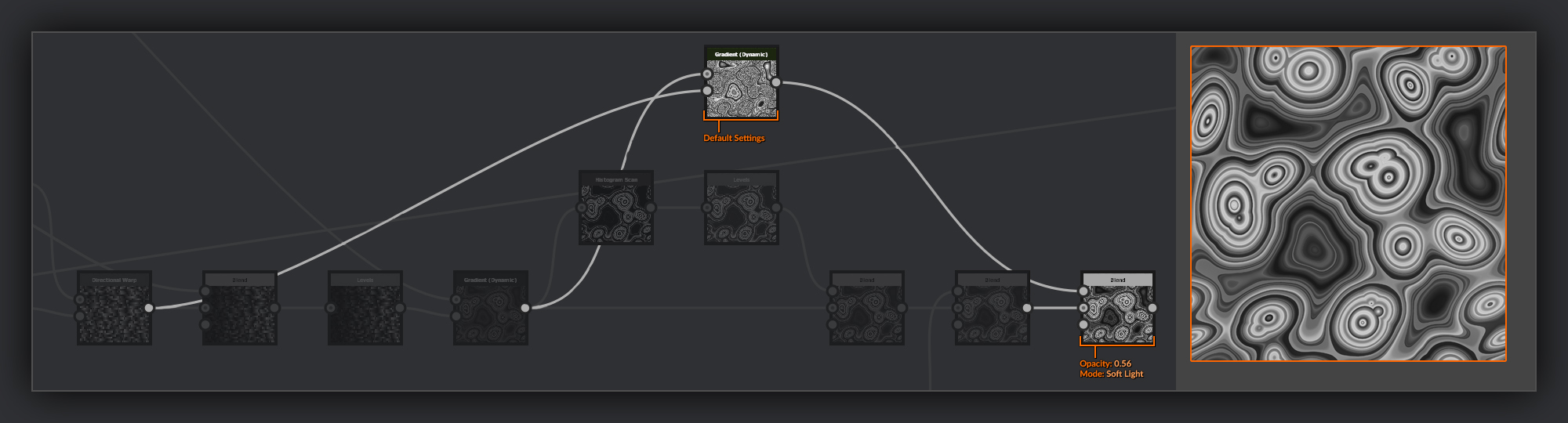
Finally, for the rings, I take the output of the Gradient (Dynamic) from before and pass it through another Gradient (Dynamic) node using my rings palette. This will create some extra fine rings. I layer these finer rings over my other rings with a Blend node using soft light and a middle opacity.
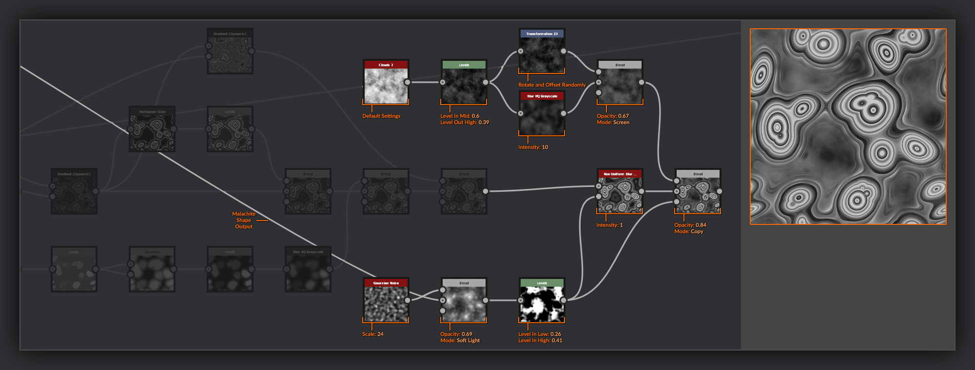
The next few steps are to add some subtle noise variations throughout the rings. Before I add the noise, however, I want to reduce the strength of the rings in the lower areas.
To do this, I create a new mask based on the valleys of malachite. I take the output of my Malachite surface and Blend it with a Gaussian Noise using Soft Light as the Blend node. I then use a Levels node to squeeze the values of this mask to isolate just the lower regions, while also inverting the output levels to invert the result. I use this new mask to blur the rings in a Non Uniform Blur Grayscale node.
To keep these darker areas interesting, I’m going to add some noise in.
I take a Clouds 2 node using Levels. I shift the midpoint in the right to bias the darker values, and then reduce the levels out to further darken the noise. I blur my output with a Blur HQ Grayscale
to remove some of the macro detail. Then I combine it with the unblurred version that has been moved with a Transform 2D node using a Blend node set to Screen to add back in some of the macro detail lost previously. This is then combined with the rings in a Blend node using Copy with high opacity, using the valley mask to prevent it from affecting the peak rings.
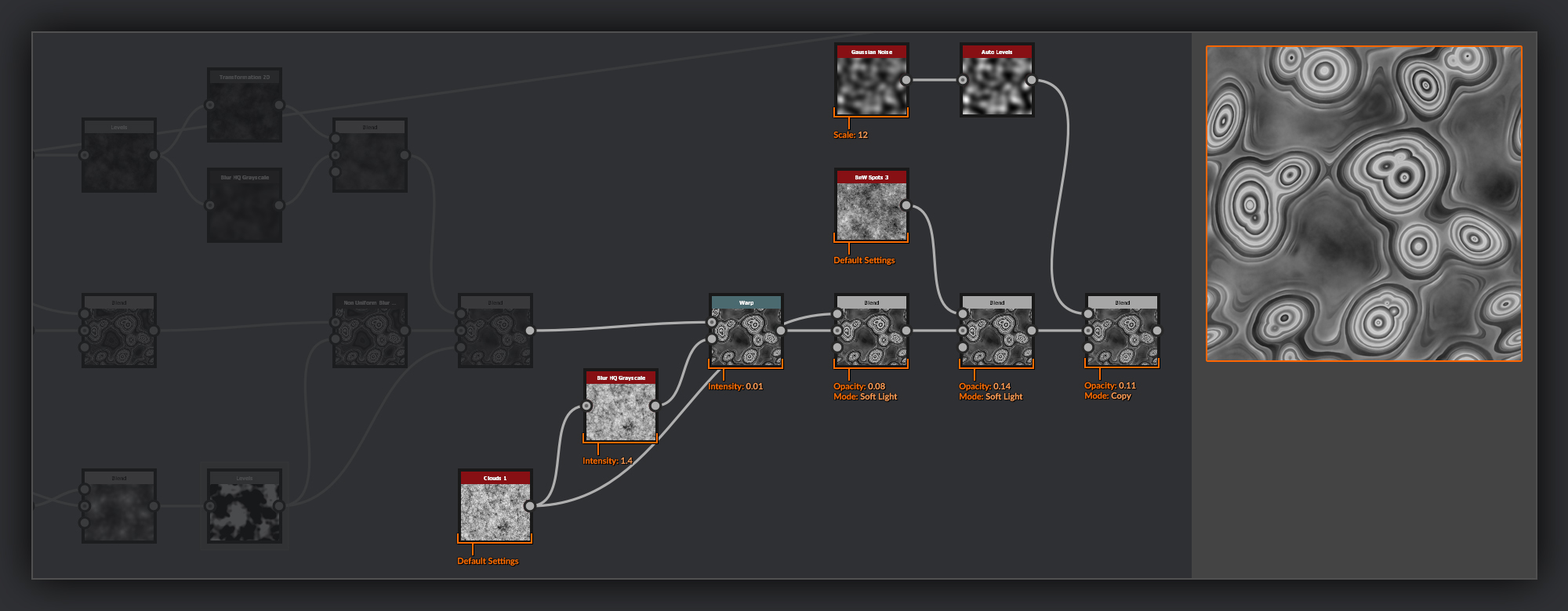
Now I’m going to start building up some subtle noise across the whole of the Malachite surface. This will help add some further detail to the rings themselves, as well as provide a few organic imperfections to help keep my result looking natural.
First I distort my rings using a Warp node and Clouds 1 that has been slightly blurred with a Blur HQ Grayscale to prevent high-frequency noises in the input. After this, I blend the unblurred Clouds 1 in separately with a Blend node set to soft light and very low opacity. Then I am going to blend in some BnW Spots 3 with a Blend node set to soft light and a low opacity. Followed by a Gaussian Noise that has been passed through Auto Levels which is combined using a Blend node set to Copy and a low opacity again. This should help shift the color around the rings, so each ring is not too monotone.
The last thing I’ll do to my rings is add some small spots around the rings that I spotted in a few samples during my research.
For these, I’ll add a Tile Sampler and use a bell shape scattered across the canvas with a lot of size and luminosity variation. I’ll then select a small range of these spots using a Histogram Scan node. I use these spots as a mask in a Blend node to blend in some more of the Clouds 1 set to Multiply with a middle opacity. At the very end I use Auto Levels on this rings pass to make sure I have a full range of values to play with as I continue.
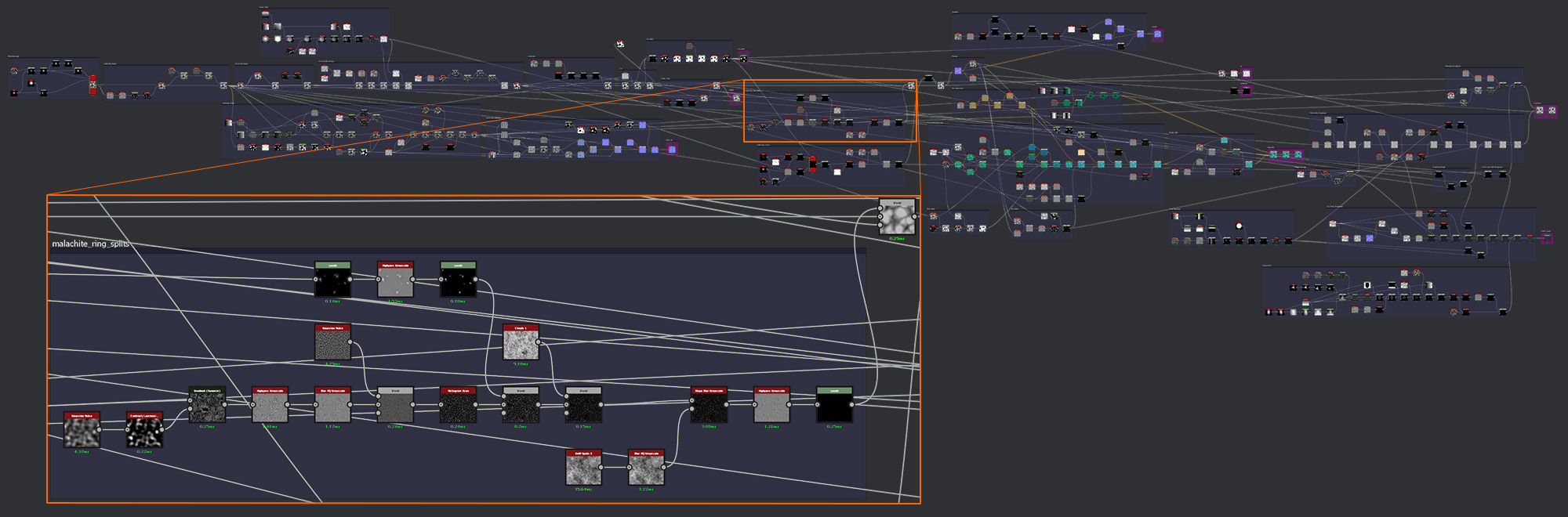
Malachite Ring Splits
Now I’ve got my rings set up for the malachite I can add a small amount of information from them into the Normal map. I’m going to take some of the recesses between the rings and turn them into gaps between the rings on the surface of the cut malachite.
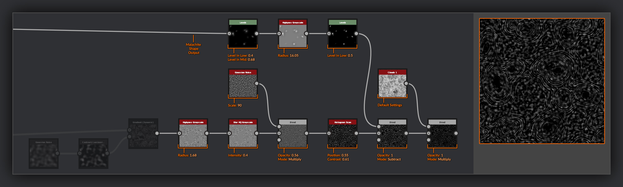
I will start by taking the output from my malachite rings and passing it through a new Gradient (Dynamic) node. For the gradient input, I am going to use a Gaussian Noise passed through a Contrast/Luminosity node to increase the contrast.
Now to set up a series of nodes to isolate some small parts of the rings to turn into splits.
The first thing I do is a run my Gradient (Dynamic) output through a Highpass Grayscale node with a very small radius. Next, I put it through a Blur HQ Grayscale node to reduce the sharpness of the underlying gradients, before combining it with a Gaussian Noise node in a Blend node set to Multiply. Then I add a Histogram Scan to isolate the highest points in the rings.
Because I want to ensure the very center of each cut face is unaffected by the splits, I create a mask by isolating the very tip of each peak from my Malachite Shape output in a Levels node. I then put this through a Highpass Grayscale node to even out the values, before putting it through another Levels node in order to bring the Level In Low back up to the midpoint. I then use a Blend node to subtract these peaks from my splits.
To add some finer noise, I finally Multiply in a Clouds 1 over the top in a Blend node.
Next up I’ll add some chips to the edges of these splits. I’ll do that with a Slope Blur Grayscale with its mode set to Min. For the slope, I use a BnW Spots 3 softened with a Blur HQ Grayscale. I then do another Highpass Grayscale pass on the output of the Slope Blur Grayscale to even out the values in my splits before finally passing them through a Levels node where I bring the level in up until just a little of each split is visible. I then reduce the level out, so the splits aren’t too deep.
With my splits finished I combine them into the output of the Small Chips frame output, using a Blend node set to subtract with a very low opacity. I mask this Blend node using the cut mask I created earlier to ensure the splits are only visible on the cut surfaces of the malachite.
Finally, I frame up my ring splits.
Malachite Cracks
In the Mattershots reference image, there are some hairline cracks radiating from the center of the cut Malachite face. I wanted to add them to my Substance texture, and have them radiating from the center in the same way.
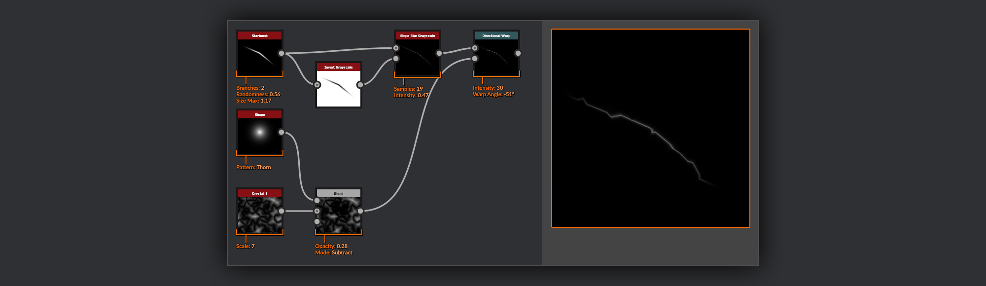
I’ll begin by making the crack shape.
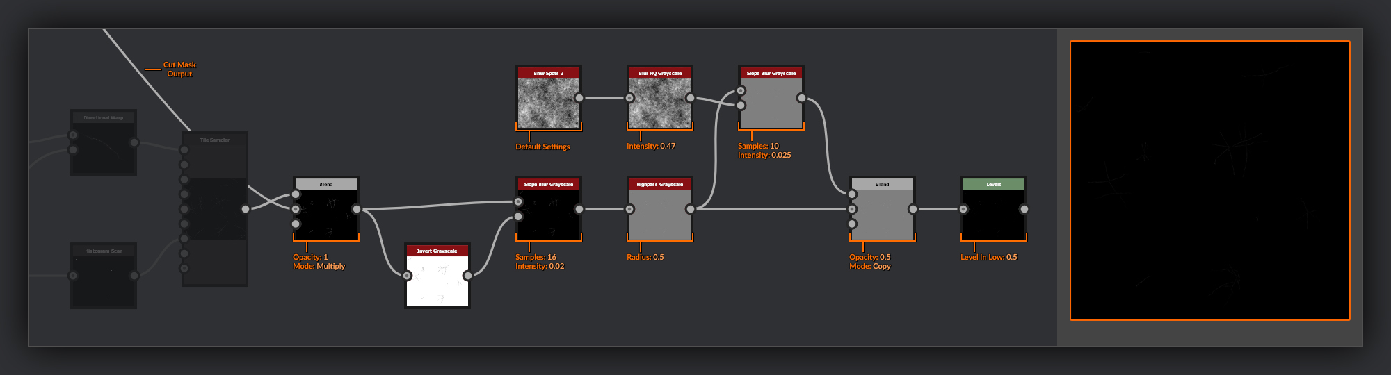
I take a Starburst and reduce the number of Branches to 2 while also increasing the randomness. This is an excellent quick way of getting a squashed ellipse shape with a kink in the middle. I put this crack shape through a Slope Blur Grayscale node the same shape put through an Invert Grayscale for the slope input. Using a low intensity, you can slide the values towards the middle of the starburst, creating a nice fine line of pixels with a small falloff.
To add some smaller irregular angles to the crack shape, I warp it using a Directional Warp node over a Crystal 1 node. To avoid shifting the midpoint of the crack away from the center of the canvas I subtract a thorn Shape
from the Crystals so that height information is removed at the center. This is important as I want my cracks to terminate at the center of each Malachite face.
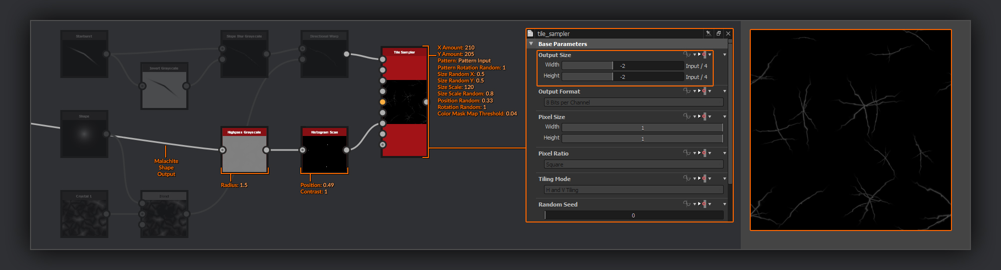
For placing my cracks, I use a Tile Sampler with my crack in the pattern input. This is one place I will recommend setting the output of the node down, as the number of cracks placed and the use of a mask makes this quite an expensive node to process. I put the scale down -2 from input in my graph.
To ensure that the cracks only appear where I want them to (from the center of my cut Malachite faces), I need to create a mask of the very tips of the peaks.
For this, I take the output of my Malachite Shape and run it through a Highpass Grayscale with a low radius. I then isolate just the very tips with a Histogram Scan. This is put into the mask input of the tile sampler.
After placing my cracks, I multiply my Cut Mask over the top of them with a Blend node to ensure the cracks don’t spread outside of the cut surface.
Next, I repeat the same Slope Blur Grayscale pass from the single crack before, with an Inverted
copy of my tiled cracks as the slope input, to again tighten up the cracks. This also helps blend the various cracks at the origin point giving them a slightly more organic appearance.
After this, I do a Highpass Grayscale with a very small radius to reduce the cracks width even further. After the Highpass Grayscale, I add in some chips as before on the Ring Splits, using a Slope Blur Grayscale and blending it back with the unchipped cracks. Finally, I add a Levels node with the Level In Low set to the midpoint, so that I only retain the information above mid gray.
I’ll frame up my cracks here, and label them accordingly.
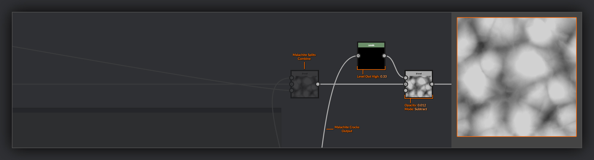
Before blending the cracks into the Heightmap, I add a separate Levels node to reduce the level out to make the cracks less intense. I often like to do passes such as this within separated nodes, as it can make managing the result easier. Setting the levels out down too low in the previous node would have made any changes I made to the levels in hard to see in the 2D preview window. With quick to calculate nodes like the Levels node, the graph render time is only slightly greater if you chain a few together. If you need the speed there’s no issue collapsing them down to a single node later in an optimization pass.
I mix the cracks into the node chain using a Blend node set to Subtract and a very low opacity.
This is the end of the chain for the cracks, so I frame it up separately to keep it clear.
Normal Map
Now I’m ready to finalize the Normal map. Usually, I don’t do much addition of information to my Normal maps that isn’t already included in my Heightmap. This graph was a little unusual in this case as I separated my Heightmap before adding the splits and cracks to the cut malachite surface, but while working on my entry for the Materialize Contest, I didn’t like how intense those features ended up looking when I left them in the Heightmap. Hence choosing to diverge a little earlier than I usually might.
I separate the Normal node from the rest of my output nodes after the Safe Transform Grayscale and bring it forward to the end of my cracks. At this point, I’ll move over my Curvature Smooth node with the Diffuse Output node, as well as creating a Curvature node, as I will be making use of this later on in the roughness and BaseColor stages. I put a frame around these few nodes to keep them visible, leaving the outputs outside for now.
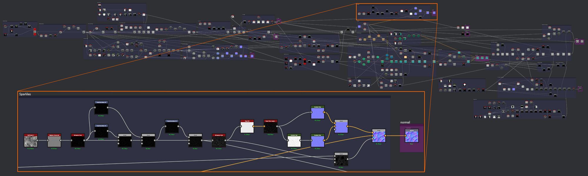
Sparkles
I felt that the surface of the chrysocolla needed a little more visual interest. I decided on adding some glittery sparkliness to the crystallized surface of the chrysocolla, something else that I had seen in a few of my researched reference images.
I start my sparkles with a BnW Spots 3 that I put through a Highpass Grayscale with a low radius to reduce the ranges, I then isolate a few spots using a Histogram Scan.
Next, I transform and layer this output in various ways to build up a dense splatter of individual dots. First with a simple Transform 2D, a 90-degree rotation, and a slight offset. I add this result in with a Blend node set to Copy and a relatively high opacity. Then another Transform 2D; this time I reduce its scale by half and again rotate and offset it in different directions. I combine this one with my sparkles with a Blend node set to Max (Lighten). Finally, I do another Transform 2D of this newly combined group of dots, again reducing it by half and rotating and offsetting it in different directions. I also combine this one with a Blend node set to Max (Lighten).
Now I want to isolate a specific selection of the spots, to turn them into proper sparkles.
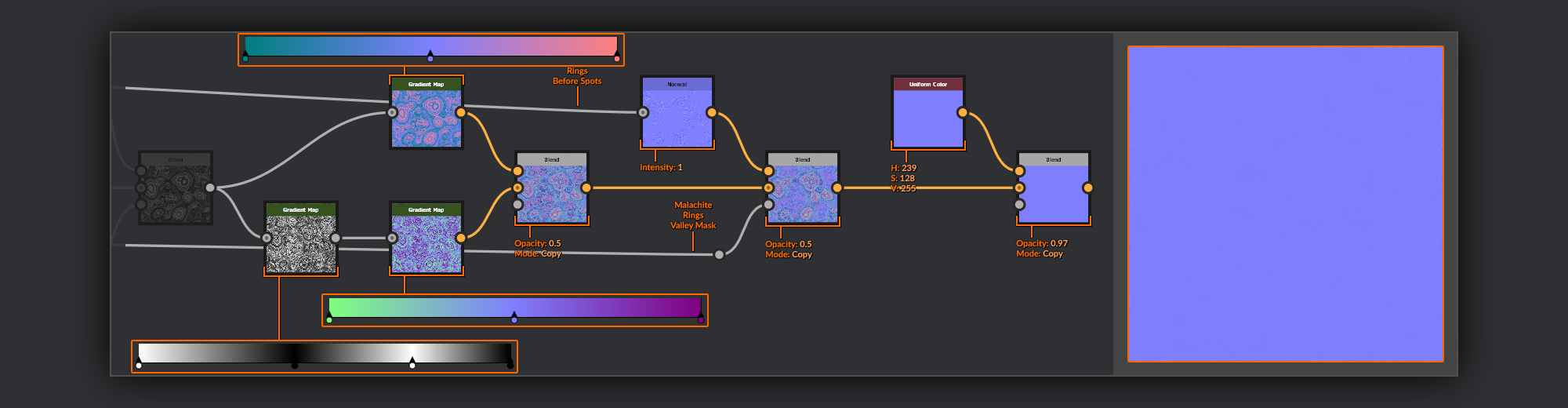
I use a Histogram Scan node to select as many of these dots as I want to turn into normal facets on the surface of the Chrysocolla. These facets mean the sparkles will catch the light at different angles and twinkle in my renders.
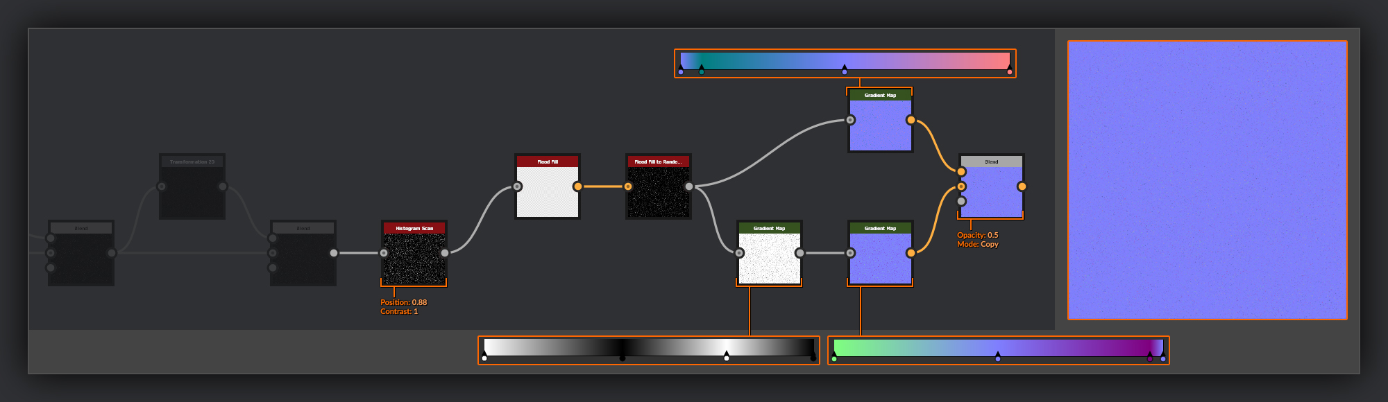
To give the facets a random direction I Use a Flood Fill and a Flood Fill to Random Grayscale to assign each sparkle its own grayscale value. I pass these flooded spots through two Gradient Map nodes to fill them with normal directions. The first gradient map handles left and right direction of various strengths. The second gradient I mix up the grayscale values of the sparkles first with a separate Gradient Map before running it through a
Gradient Map handling the up and down normal directions. I make sure to keep the space between sparkles flat normal so they don’t interfere with my overall Normal map at the edges of each sparkle.
These two normal direction passes are then blended together using a Blend node with an opacity set to 0.5 This blend will give me sparkles with a chance of facing in every possible normal direction.
If you’re not as obsessive as me to have memorised the RGB values for each Normal map direction, a very quick way to find pretty accurate values is to create a Shape node with a Pyramid shape or a Polygon 2
with 4 sides and then hook this into a normal node with a super high strength, like 9000, to get pure directional colors. You can then pick from what you see in the normal from the 2D view to build your gradients.
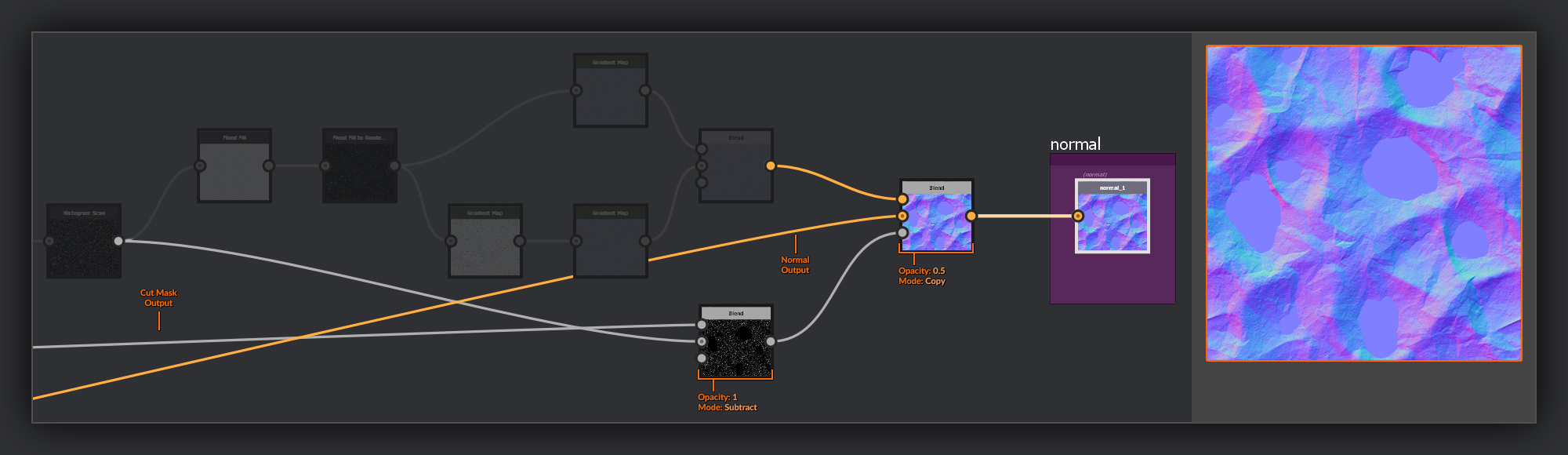
I combine this sparkles Normal map with my Malachite Normal map, using a Blend node set to Copy with the opacity set to 0.5. I don’t want to completely override the underlying surface, otherwise the sparkes appear to float or stand proud of the surface below. Finally I make a mask by removing my Cut Mask output from the Sparkles histogram output in another Blend node
set to subtract. I put this new mask into the mask input of my Normal Map Blend node. This prevents sparkles from appearing on the cut Malachite surface, but also stops the spaces between the sparkles from flattening my underlying Normal map.
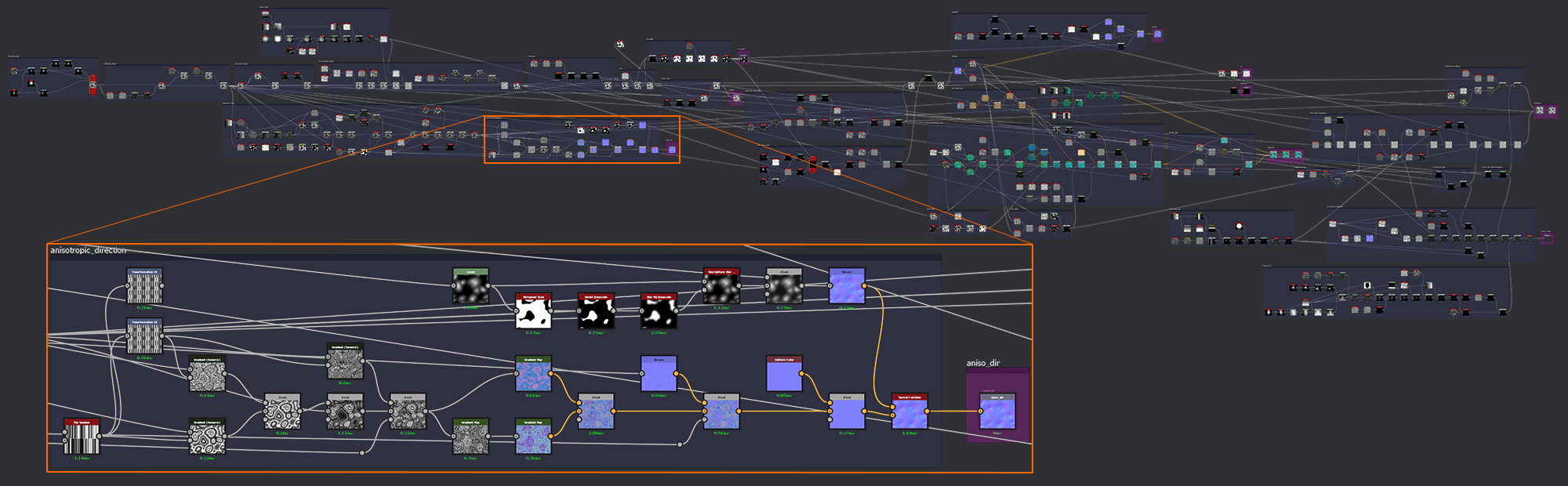
Anisotropic Direction
To make full use of the anisotropic shading available in MDL I need to create a map that will define the direction of my anisotropic highlights for each of the cut faces. The base shape will be the output from the Malachite Shape frame, but on top of this I will add some variation driven by the individual rings of the cut malachite.
First, I’m going to create some rings of normal information that I will use to add slight directional variation to the rings of the malachite.
I begin by creating a new palette from which to create some grayscale values that I will use to drive my ring selections. As in the Malachite Rings previously I make a Tile Random node; I use the default square shape and set the Color Random variation to full.
Now to make the rings.
I create 2 Gradient (Dynamic) nodes using the Malachite Surface output as the source for their grayscale input. In the first I use my previously created palette as the Gradient input. For the second I take the palette and reduce its size by 4 in a Transform 2D to get some finer grayscale bands. I then combine these finer bands over my larger bands using a Blend node set to Copy with a very low opacity.
This is the start of a Heightmap for my anisotropic direction map.
Next I’ll combine some of the information from my Malachite Rings frame with my anisotropic direction Heightmap.
First I’ll combine the anisotropy Heightmap with my Malachite Rings, I use a Blend node set to overlay to achieve this. Next to add some bands to the lower areas of the Heightmap between the peaks, I create a new Gradient (Dynamic) node and use the Malachite Rings Heightmap as the grayscale input; for the Gradient Input I use my scaled-down palette. I add this into my anisotropic direction Heightmap using a Blend node set to Copy. I use the valleys mask I created for the Malachite Rings as a mask to constrain these noisier bands to just the valleys between the peaks.
Now I’m ready to convert these rings into the Normal map direction information that the Anisotropic map will need. I’m going to use a very similar method to the sparkles before.
First I pass the rings through a Gradient Map node filled with left and right normal direction information. For the second pass I first mix up my grayscale map with a Gradient Map node filled with a couple of black and white points to shuffle the order of the rings. Then I pass this gradient output into another Gradient Map node filled with up and down normal information. The outputs of these two gradient maps are then combined with a Blend node set to Copy and a 0.5 opacity.
To soften up the valleys a little I take the output of my Malachite Rings and run it through a Normal node with an intensity of 1. I then combine this with the start of my Anisotropic Direction normal using a Blend node set to Copy with an opacity of 0.5 again. I use the valleys mask from the malachite rings to make sure it doesn't cover the peaks. Finally to reduce the overall strength of the normal information in my rings I blend in a flat normal color using a Blend node set to Copy with a high opacity. This is to stop the anisotropic highlight from spreading too far around the rings, I only want a small variance in direction in each ring.
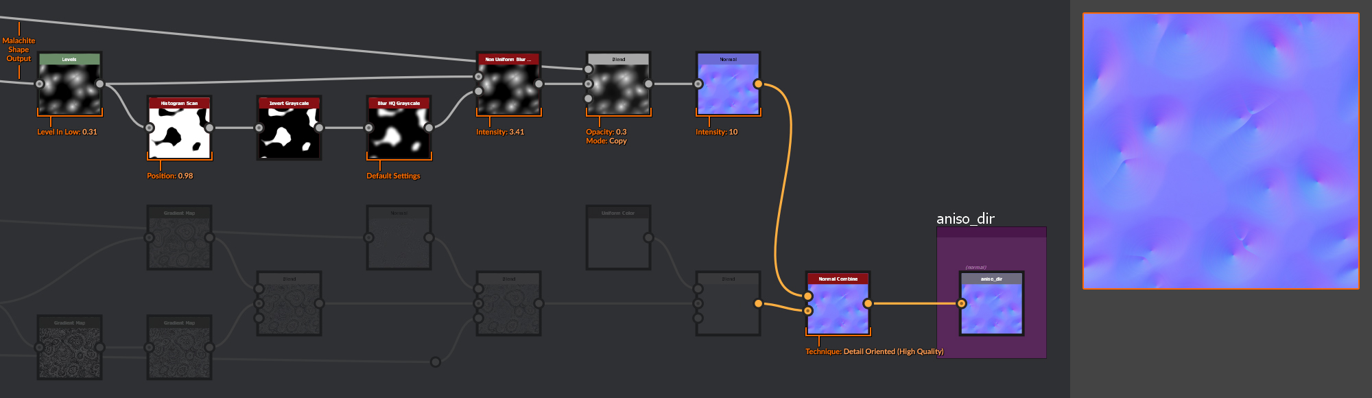
Now I want to add the normal layer that will handle the bulk of the anisotropic direction work.
I start by taking the output of my malachite Shape. I add a Levels node and raise the level in to cut out the valleys and isolate the peaks. Using an Invert Grayscale node followed by a Histogram Scan node I create a mask for the valleys. I then soften this with a Blur HQ Grayscale node. In a Non Uniform Blur Grayscale node I use this mask as the blur map input, with my isolated peaks height fed into the grayscale input. I blur my peaks to remove the sharp transition from grayscale gradient to black at the base of each peak; the mask helps to prevent blurring the tip of each peak.
I then combine this with the output of the Malachite Shape height, using a Blend node
set to Copy and a low opacity to bring a little height information back to the valleys, ensuring they aren’t completely flat. I pass the output of this into a Normal node, before combing it with the rings Normal made previously using a Normal Combine node set to Detail Oriented (High Quality). Finally I add an output node for my anisotropic direction map and frame it up separately to keep it visible.
I’ll also now frame up the rest of the nodes making up my anisotropic direction map.
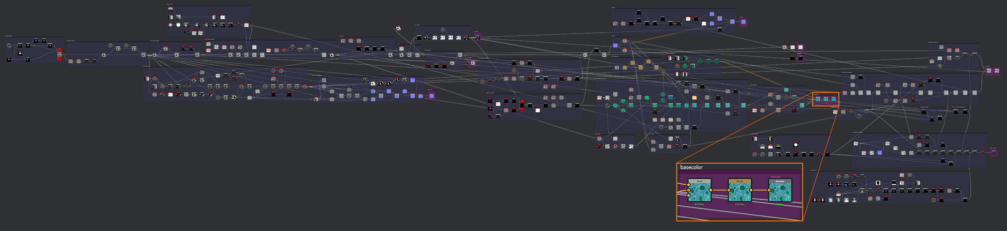
Basecolor
Now I have both my Normal maps and Heightmap taken care of it’s time to start putting some color down. I need to create BaseColor maps for two individual surfaces, the outer Chrysocolla layer and the cut faces of the Malachite. These will then be combined with the cut mask to give us a complete BaseColor. I’ll use gradients a lot for generating my colors, mixing them with various outputs from the rest of the graph to combine the various surface details.
Chrysocolla Base color
I’ll start with the Chrysocolla as it comes first in the Heightmap chain.
Let’s begin with the Chrysocolla as this takes up the majority of the surface.
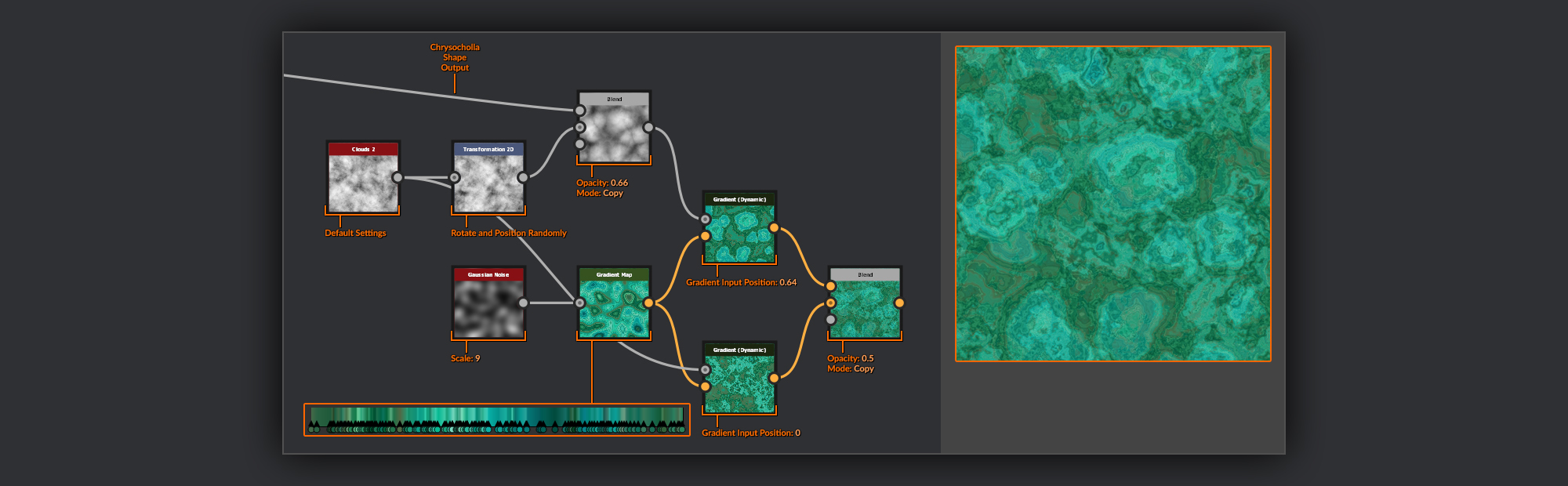
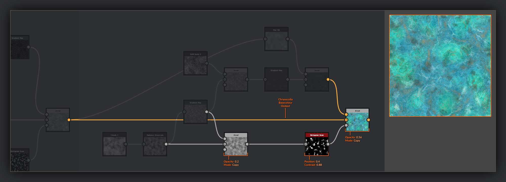
As I’ve often done before I’m going to start by creating a palette from which I will grab the colors for the base of my Chrysocolla. I create a Gaussian Noise node and connect it to a Gradient Map node. In the Gradient Map node I select some colors from my reference images. For now I focus on the greener areas. You can see in the references how the chrysocolla is a mixture of turquoise and blue tones. The blue is often found in recess away from extremities where it appears it may be rubbed off so I’ll add that blue layer later.
In the first of two Gradient (Dynamic) nodes I use a plain Clouds 2 node as the Grayscale Input. In the second Gradient (Dynamic) node
I take the output of my Chrysocolla surface and combine it in a Blend node with the Clouds 2 node that has been passed through a Transform 2D node giving it a random position and rotation. I use a different Gradient Input position in this second Gradient (Dynamic) node to ensure I have some different color values selected from the palette. I then combine these two Gradient (Dynamic) outputs together in a Blend node using a 0.5 opacity.
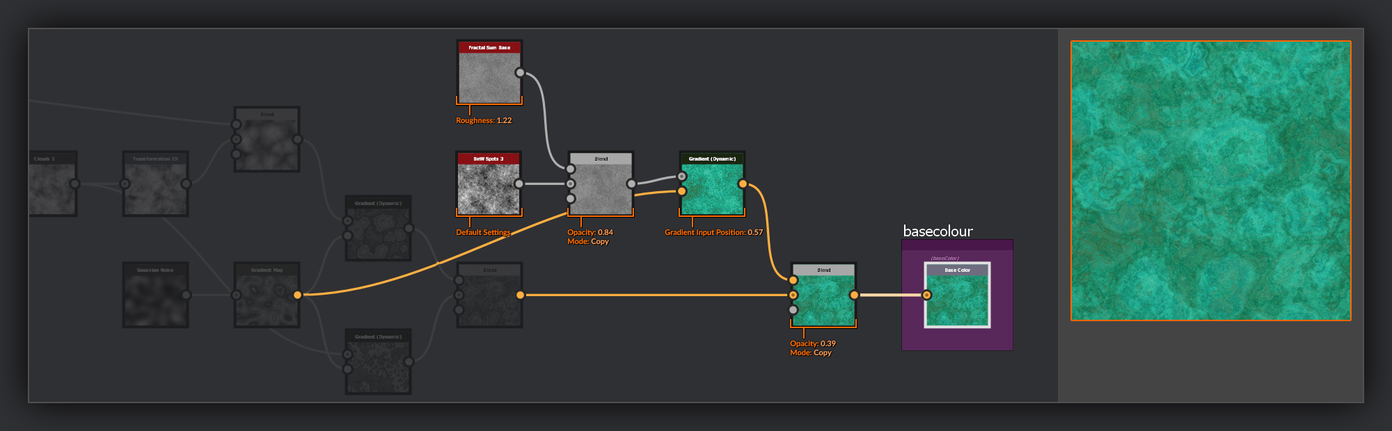
For the final Gradient (Dynamic) node I combine a BnW Spots 3 with a Fractal Sum Base in a Blend node with a high opacity to get some mixed up high frequency noise. I then use a
Blend node again to combine this noise with the previous two using a 0.38 opacity.
This is a good moment to take the BaseColor Output node from where I left it with the Curvature nodes and swap it over from the Uniform Color grayscale to this new chain so I can see the changes I’m making in the 3D view. I’ll move it along with me as I go until the BaseColor is wrapped up.
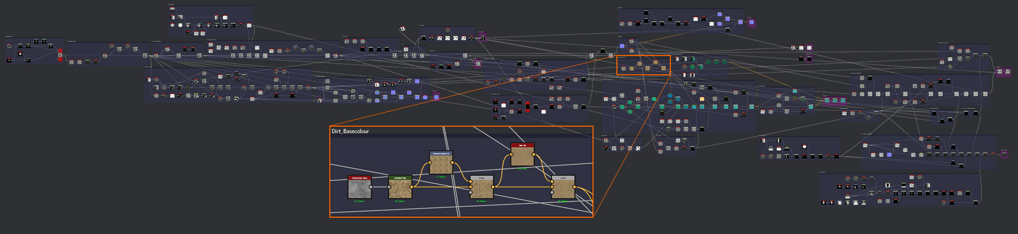
Dirt Basecolor
I want to add some sandy veins to the surface of my Chrysocolla so now is a good time to quickly make a frame to hold a dusty noise.
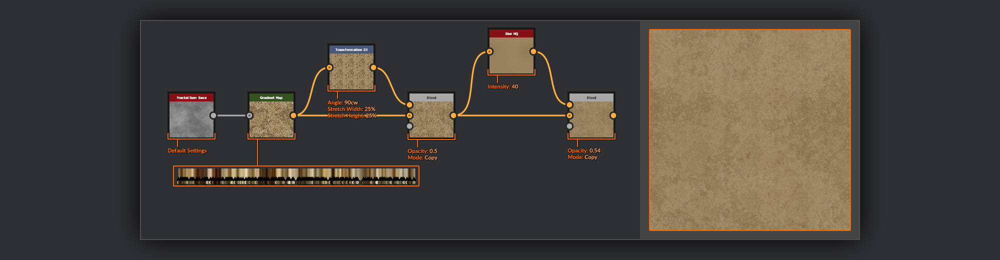
This is pretty straightforward. I take a Fractal Sum Base node and pass it through a Gradient Map node filled with various sandy colors. Then, using a Blend node set to 0.5, I combine this output with a version of itself tiled a few times using Transform 2D node. This helps reduce the contrast in the final output while also adding some macro variation to the noise.
After this I combine this output with a copy that has been passed through a Blur HQ node to get an average of the dust color; again I use a Blend node
with the opacity set to the middle. This helps reduce the noisiness of the dust, as well as even further reducing contrast.
Back to Chrysocolla Basecolor
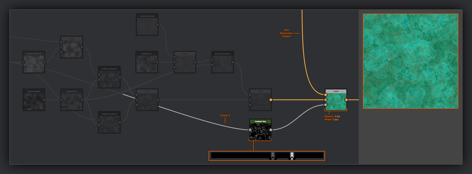
Back in my Basecolor node string I blend this dirt into the graph using a Blend node set to Copy. For the mask of the Blend node I create a Gradient node with the Clouds 2 node as the input; in this Gradient node I define a couple of fine bands of gray and white where I want my sandy veins to appear on the surface.
Blue Mask
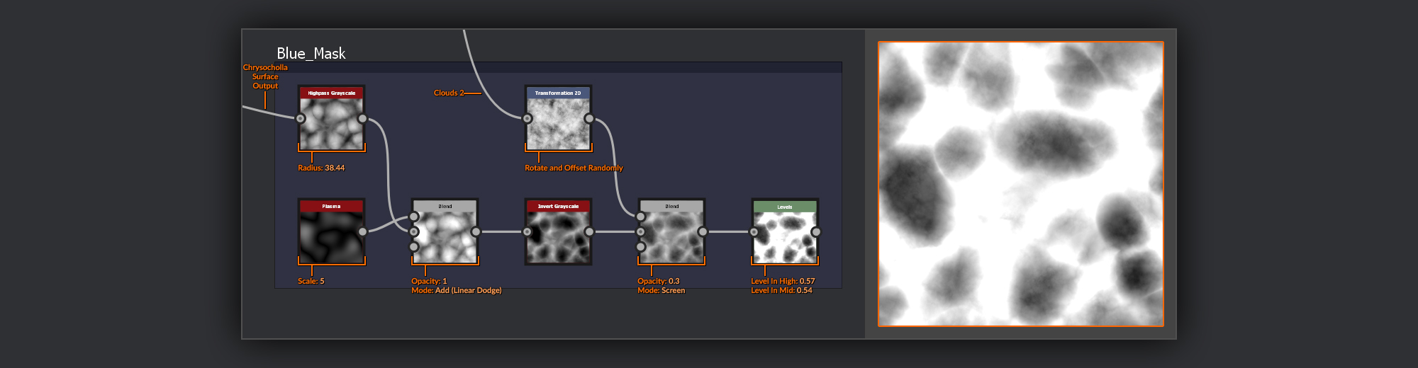
Now it’s time to add the blue bloom I spoke about earlier to the recess of the Chrysocolla. The first thing I’ll need is a mask that I’ll use to define exactly where I want the blue to appear.
I’ll take the output of my Chrysocolla Surface Frame and plug it into a Highpass Grayscale node
to level out the values a bit, as I want the bloom to appear pretty evenly between the peaks, not just in the very lowest recesses. I combine it with a Plasma node using a Blend node set to Add (Linear Dodge) before Inverting it in an Invert Grayscale node. Then I combine it with another Transform 2D node manipulated instance of the Clouds 2 from my Chrysocolla Basecolor in a Blend node set to Screen. Finally I use a Levels node to adjust the Level In High to determine how high up the peaks I want the bloom to appear.
I’ll leave this mask in its own frame outside of the Chrysocholla Basecolor.
Back to Chrysocolla Basecolor
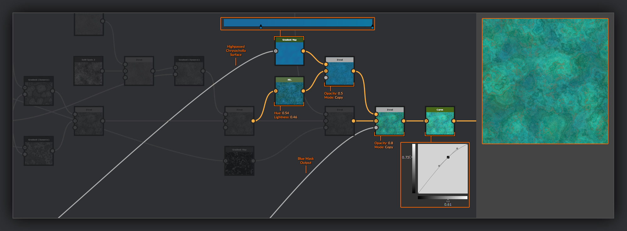
Because the blue layer is only a thin coating I’ll take most of my color noise from the underlying Chrysocolla BaseColor, simply shifting the hue towards blue and then adding in a slight gradient that gets darker as you move towards the recess in the valleys between the peaks.
To start the blue coloration I put a copy of the Chrysocolla Basecolor through an HSL node to shift the color more towards blue and to darken it a bit. I also create a new Gradient node, and use the Highpassed Chrysocolla Surface from my Blue Mask as the Grayscale Input. I set the gradient colors to two similar blue values that are darker on the left to keep some depth/height influence in my blue shades. I combine these two color layers in a
Blend node set to Copy with a 0.5 opacity. This is going to give the bloom a softer appearance to that of the rocky areas, as copying over the simple gradient will help lower the contrast in the noiser Chrysocolla layer.
I then combine this Blue layer into my Chrysocolla Basecolor string using a Blend node set to Copy with a high opacity. I use the Blue mask created previously as the mask input. Before moving on I make a quick adjustment to my overall color intensity and brightness using a Curve node to bring the mids up slightly.
Dirt Mask
Now I’ll add in some more of the dirt color I made previously. I want to keep this dirt confined to the bottom of the valleys between malachite peaks where it might collect naturally. Above the valleys it will probably have been removed by handling.
To do this I’ll need a mask that features these crevices between the peaks of my Chrysocolla surface.
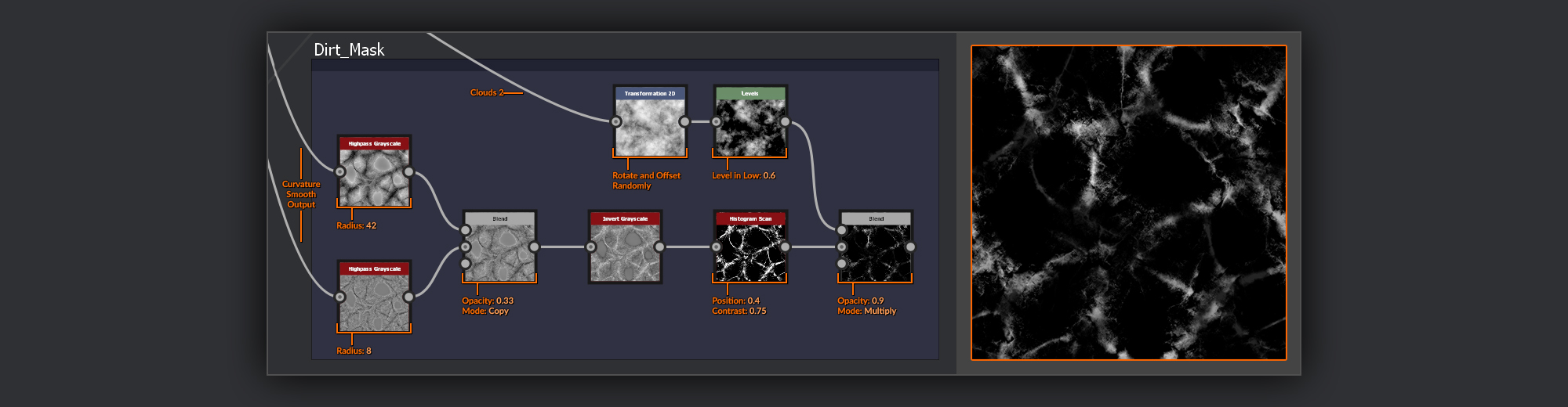
I create a pair of Highpass Grayscale nodes which both use the Curvature Smooth nodes created with my Normal map as their input. In one I set the radius to 42 and in the other I set it to 8. I then mix the 42 radius instance over the 8 in a Blend node
set to Copy with 0.33 opacity. Adjusting this blend later can quickly give me control over how far the dirt will spread. I then pass the output through an Invert Grayscale and into a Histogram Scan where I isolate just the level I want dirt to appear.
As a last step I take yet another Transform 2D node manipulated instance of the Clouds 2 from the Chrysocolla Basecolor and using a Levels node I bring up the Levels In Low, before layering it over my dirt mask using a Blend node set to Multiply to make sure the dirt isn’t too evenly distributed across the Chrysocolla.
Back to Chrysocolla Basecolor
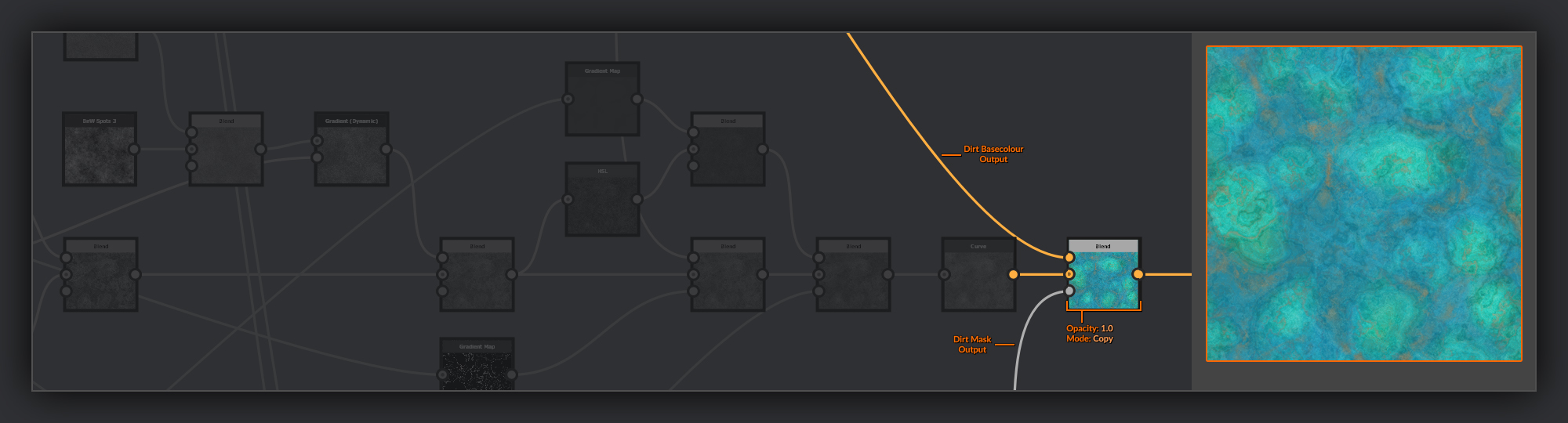
Back in the Chrysocolla chain again, I combine the Dirt Basecolor into my Chrysocolla Basecolor using a Blend node with the dirt mask from the previous section in the opacity input.
It’s not overpowering, and will be somewhat concealed by the AO, but details like this help add believability to materials. People often find grimy things look more natural in 3D; it’s much harder to create convincing pristine surfaces.
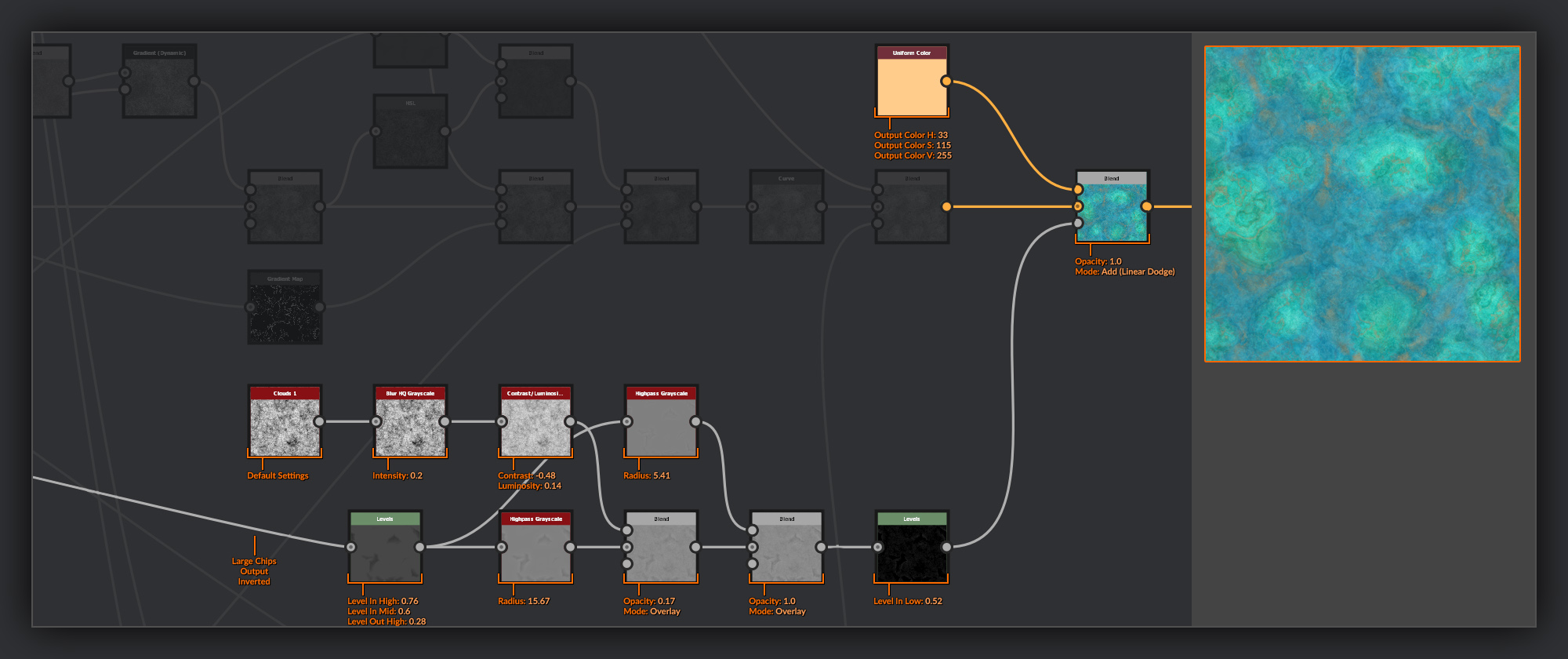
Next, I want to add some paleness to all but the depths of the large chips I added to the surface of my chrysocolla, as if the surface exposed by the damage is fresher and slightly less weathered.
To do this I create a simple mask based on the inverted output of my Large Chips frame. I put this through a Levels node that reduces the Levels in High so that only the lowest points remain dark. I also bring the Levels out High down to reduce contrast in the values. I then pass this through a Highpass Grayscale node with a radius of 15. Because of the contrast in the input this has the effect of adding a glow around the recesses to help accentuate the edges.
Next I create some simple noise using a Clouds 1 node, slightly softened in a Blur HQ Grayscale, followed by a
Contrast /Luminosity Grayscale node where I reduce its contrast by half and slightly increase its luminosity. I combine this with my Highpass output in a Blend node set to overlay with a 0.17 opacity. Then I perform another pass on the Levels node output run through a Highpass Grayscale node set to a radius of 5.5 and add a Blend node set to overlay, that helps to further enhance the edges.
Finally I add a Levels node and bring the Level in Low up to the midpoint to cut out anything below mid gray. In my main Chrysocolla Bascolor chain I use this as the Opacity input of a Blend node set to Add (Linear Dodge) with a pale tan Uniform Colour node in the foreground.
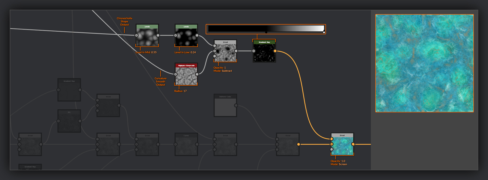
The last pass I do for my Chrysocolla BaseColor is to add some pale highlights to all of the most prominent edges, where they have been scraped or otherwise roughed up. I’ll do this with a few passes using the curvatures from the Normal I made before.
First I’ll take the output of the Curvature Smooth and plug it into a Highpass Grayscale node with a radius of 17. This ensures I’ll be getting more of the prominent edges highlighted and not just the tips of the peaks. Because I only want this highlight to show on the sharp edges, I’ll mask it from the tops of my smoother malachite nodules. For this I’ll take the output of my Chrysocolla Shape and pass it through a couple of levels adjustments.
In the first Levels node I increase the Levels in Mid to bend the values slightly towards the darker recesses. Next I pass it through another Levels node where I bring up the Levels in Low value to isolate just the higher regions of the nodules. I then combine this levelled pass into the Highpass grayscale with a Blend node set to Subtract.
Finally I add a Gradient Map node to convert the grayscale to color information and bring the black point up to the middle so that I only get the peaks. I add this to my Chrysocolla BaseColor using a Blend node set to Screen.
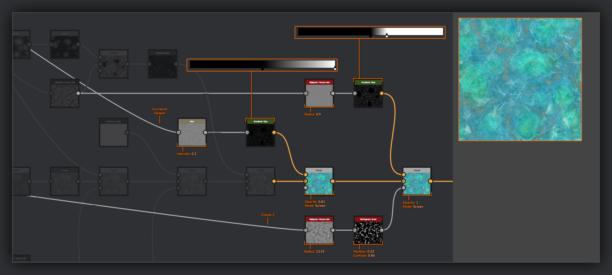
Now I’ll do a couple of similar passes, this time however the objective is to add some finer highlights.
For the first I take the output of the Curvature node (not Curvature Smooth) and put it through a Blur node with a radius of 2 to reduce the sharpness of the curvature output. As with the previous step I put it through a Gradient Map node with the same settings as before adding it to the Chrysocolla BaseColor using a Blend node set to Screen.
In the second pass I take the output of my Highpassed Curvature Smooth and put it through another Highpass Grayscale node with a very small radius. I then put this into a Gradient Map node
again, but this time as well as bringing up the black point, I also bring down the white point to increase the contrast. As before I add this to my Chrysocolla BaseColor using a Blend node set to Screen. This time with the opacity reduced slightly, I also mask this pass using the clouds 2 put through a Highpass Grayscale node with radius of 13.5 and then contrasted in a Histogram Scan node to just select just a few patches for this stronger highlight.
At this point I frame up the nodes for my Chrysocolla Basecolor.
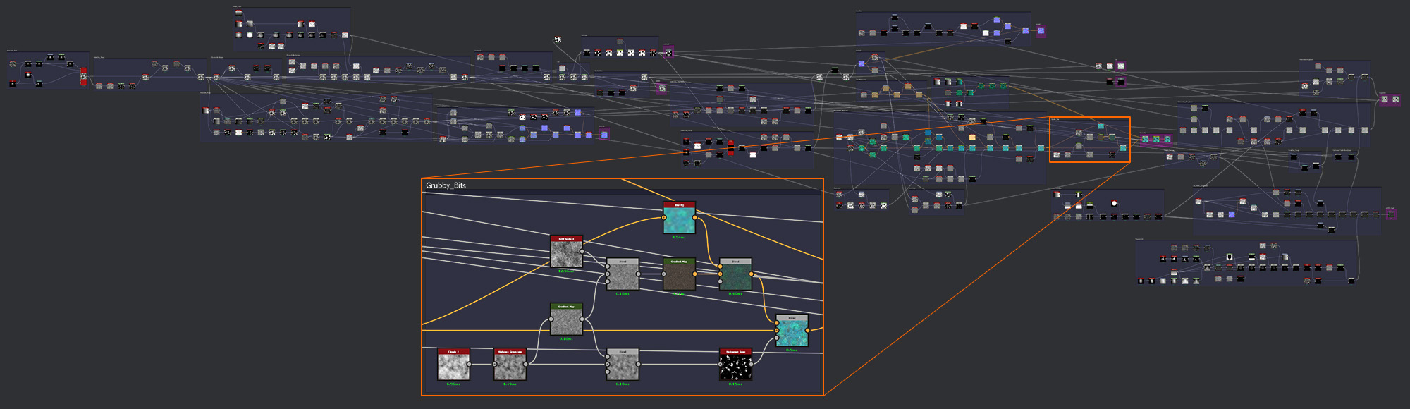
Grubby Bits
In the Mattershots reference the Chrysocolla has some darker gray-brown patches that appear to lie beneath the outer layers. I want to mimic that in my material so I’ll add them here.
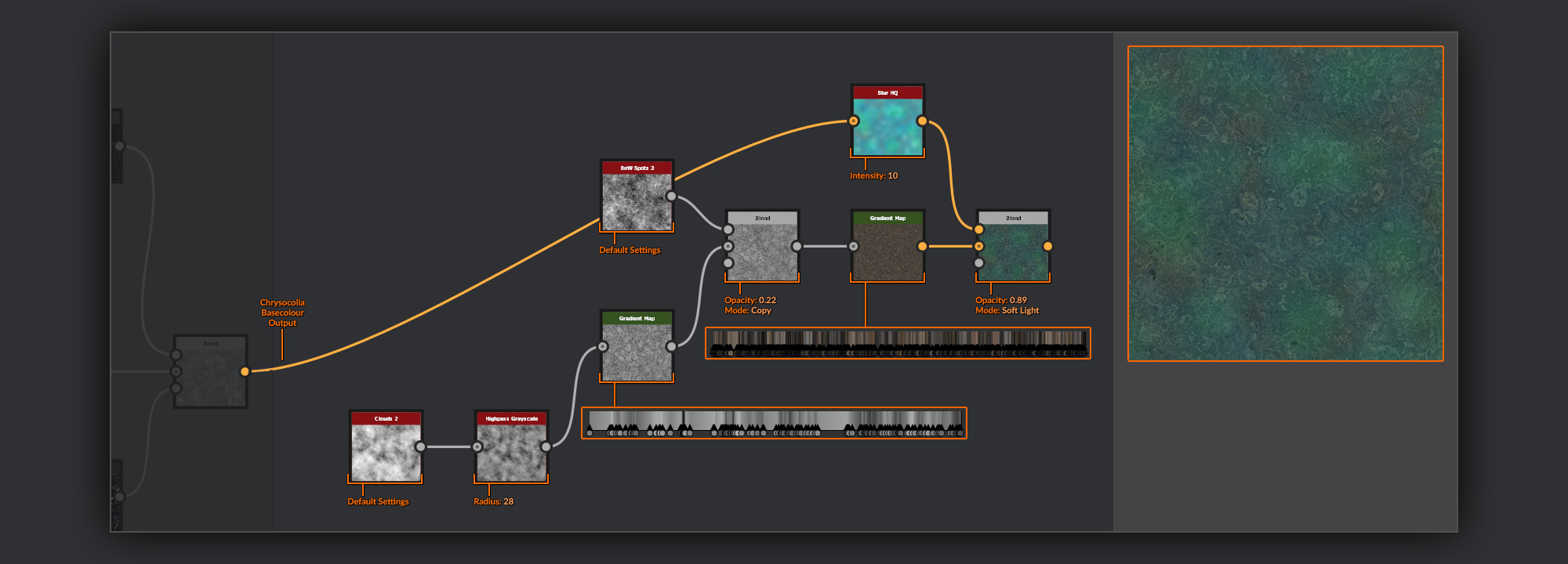
First I create some noises from which to drive an albedo for the grubby patches. I start with a Clouds 2 node and put it through a Highpass Grayscale node with a radius of 28 to even out the values. I then pass this through a Gradient Map node filled with some grayscale values to get various bands of information. To slightly break up these bands I combine it with a BnW Spots 3 in a Blend node set to Copy. I put this output through another Gradient Map node
, this time filled with some darker shades of gray and brown.
To give this the slight translucent feeling I want I’ll add in some color information from the Chrysocolla below. I combine it with a version of my Chrysocolla BaseColor softened in a Blur HQ node; this is added using a Blend node set to Soft Light.
Next, before combining this grubby BaseColor with my Chrysocolla BaseColor, I’ll create a simple mask.
For this mask I’m going to combine the grayscale bands I made previously with the highpassed Clouds 2 in a Blend node
set to Copy with a low opacity. Then I add the grubby patches to my Chrysocolla in a Blend node, with the Chrysocolla BaseColor in the background and the grubby BaseColor in the foreground. I use copy with a middle opacity, with the mask I just made in the opacity input.
Malachite Color
With the Chrysocolla taken care of I now need to make the BaseColor for the cut surfaces of Malachite which will make up the other half of my final BaseColor.
As I expect you might be familiar with now, my first port of call is a palette that will contain a few shades of green with which to color my Malachite bands.
I start with a Gaussian Noise node put through a Gradient Map with some various green and teal colors picked out.
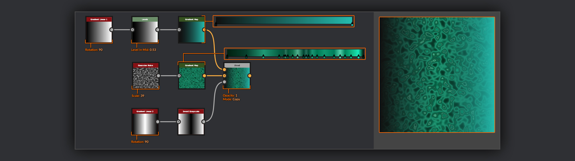
Because I want to retain the dark to light balance I’m going to mix a more straightforward gradient of dark to light values in over the top. To make this gradient I start with a Gradient Linear 1 node which I put through a Levels node
and shift the Levels In Mid up a bit to bias it slightly towards the darker values. Finally I pass this through a Gradient Map with a simple dark green to light teal gradient. I combine this with my gaussian gradient using a Blend node set to Copy, for the opacity input of the blend I make a Gradient Linear 3 and invert it with an Invert Grayscale.
This masked gradient addition means I’ll get some pretty smooth dark and light bands in my malachite, while also keeping some noisier bands in the middle of my height range.
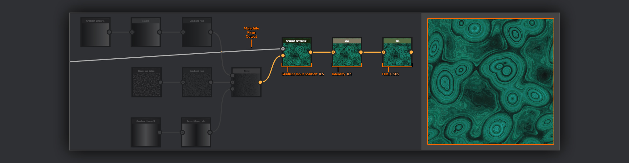
To actually colorise the rings I create a Gradient (Dynamic) node
; for the grayscale input I take the output of the Malachite Rings frame. In the gradient input I use my previously created palette. I then slightly soften the resulting gradients pixel noise with a Blur node and a very small 0.1 intensity.
Finally in my graph I’ve ever so slightly shifted the Hue of my malachite towards cyan using an HSL node. It’s easier to tweak the value precisely here than it is to go back and edit the previous gradients themselves.
Finishing the Basecolor
Now I’ve got both of my surfaces taken care of, I need to combine the Malachite BaseColor with the Chrysocolla BaseColor.
I do this with a Blend node; I use the Cut Mask from earlier in the opacity input to mask the two surfaces from each other. I add a Sharpen node with a 0.3 intensity just to crisp up my BaseColor a bit before adding an Output node.
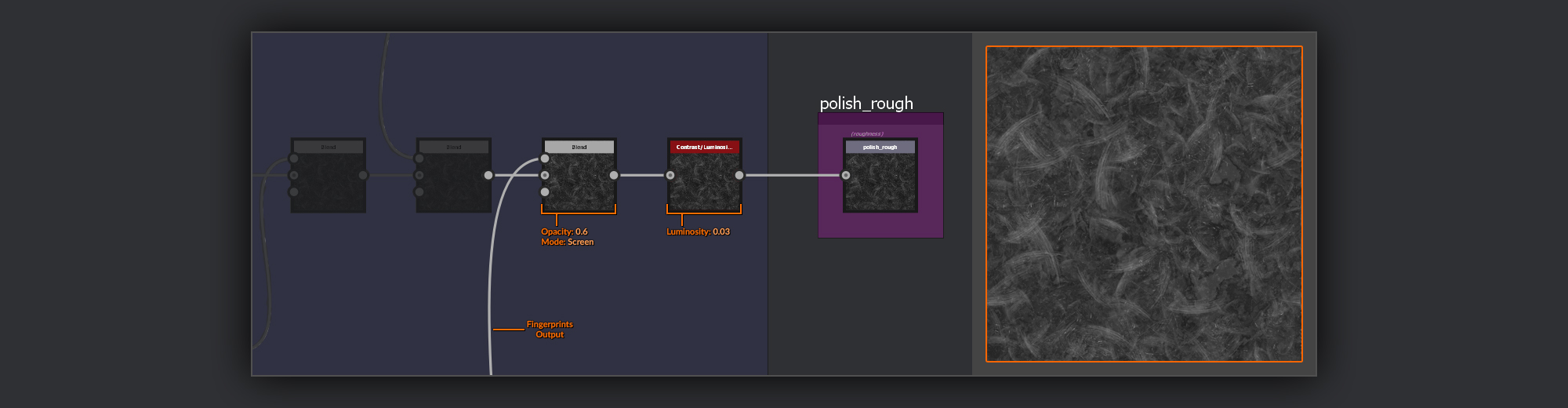
Roughness
Now we’re going to start on the Roughness map. For me the Roughness is one of the most important parts of a material, and is a really handy map to use for adding extra interest to a material. While the BaseColor does a lot of the heavy lifting when a surface is viewed front on, it’s the Roughness in combination with a good Normal map that helps keep a material interesting when viewed from all angles. Like the BaseColor, in most cases, I’m looking to create some nice contrast in my Roughness maps. Glossy surfaces can benefit from matte patches where the surface may have been worn away. Or a matte wall might have damp patches that will glisten in the right lighting conditions.
The roughness for my Malachite with Chrysocolla will be composed of a few separate passes for each surface, like the BaseColor before it. These individual passes will be combined to give us a complete Roughness. Unlike the Basecolor, where one texture contained all my color information, for my Roughness pass I’ll be making two separate Roughness maps. The first will be for the mineral itself, composed of the Chrysocolla and the Malachite. The second extra roughness will be a special texture created to look like a coat of polish applied to the surface of the cut Malachite faces. This polish coat will be utilised in the MDL to add an extra layer of information to the final Malachite with Chrysocolla renders.
My Roughness process usually begins with gathering information added in the previous steps. I’ll take information from the Heightmap through to the BaseColor to ensure it is accurately represented. Then I’ll begin layering in some unique details to give the completed piece a smattering of extra interest not present in the other maps.
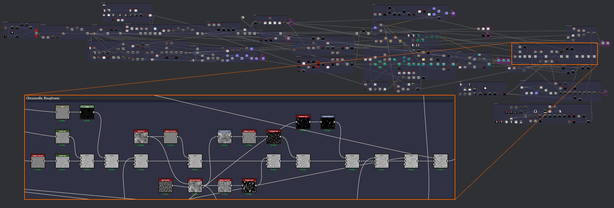
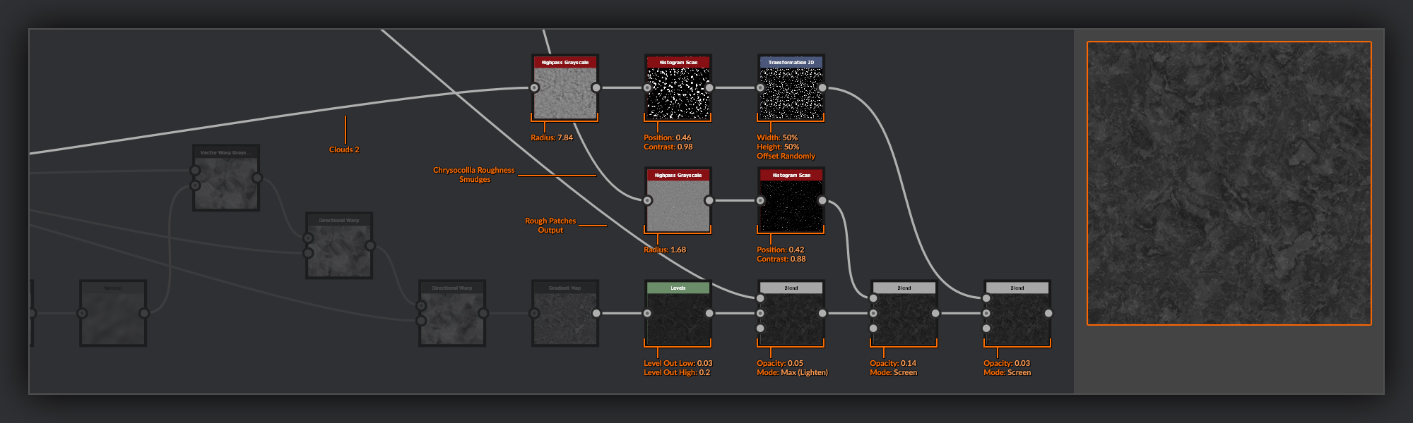
Chrysocolla Roughness
As I have done in the other steps before this, the chrysocolla is going to be first up for the Roughness treatment.
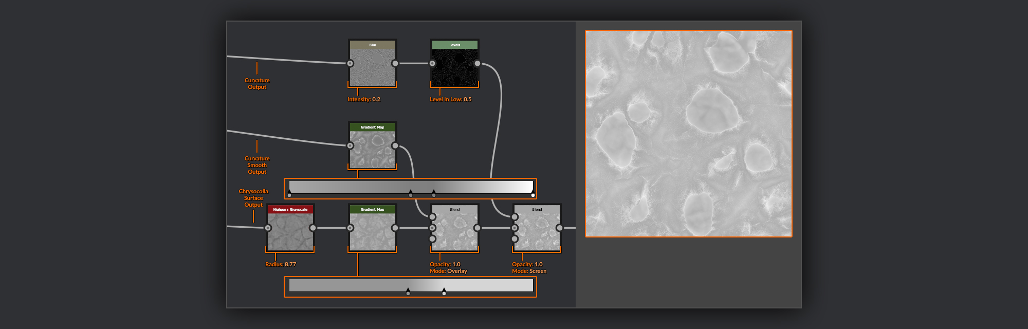
I begin by taking the output of my Chrysocolla surface and put it through a Highpass Grayscale node
with a low radius to reduce the contrast and accentuate the raised edges slightly. Next I plug it into a Gradient Map node where I’ll constrain my highest points from the rest of the graph to divide the exposed rough surface and the slightly more sheltered lower areas in the valleys between nodules. I use brighter grays here, as in general I want the Chrysocolla to appear rougher than the Malachite.
As with the BaseColor, now I change my roughness Output node over to my new roughness string so I can see what I am doing. I then take the Curvature Smooth from the Normal map and put it through another Gradient Map node. In this gradient I assign some values to highlight the highest edges, as well as to bring up some roughness in the very lowest areas of the graph. I combine this into my chrysocolla Roughness chain in a Blend node
set to overlay. After this I take the output of the standard curvature and soften it slightly in a Blur node and pass it through a Levels node, where I bring up the level in low to cut out all values below the midpoint. This I combine with the chrysocolla Roughness chain in a Blend node set to Screen.
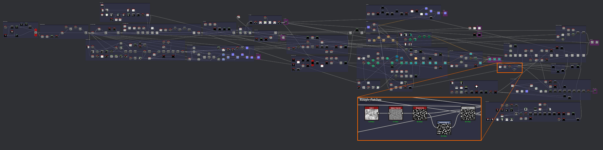
Rough Patches
To break up the uniformity of the Roughness values across the surface I’m going to create random grayscale patches of various sizes. As I’ll probably find a use for these again later in the polished surface, I’ll create the nodes for these in another separate frame to keep things organised.
I begin with a Clouds 2 node which, as done many times before, I then put through a Highpass Grayscale node to level out the values. I then use a Histogram scan node to select a slice of values from the clouds. In a Transform 2D node I’ll apply some random translation and rotation to the clouds slice, before blending it back into the vanilla version in a Blend node
set to Copy.
Back to Chrysocolla Roughness
I combine the output of my Rough Patches into the Chrysocolla Roughness string with a Blend node set to Overlay with a low opacity. I want these to break up the surface with patches of varying roughness, but only subtly.
The next thing I’ll do is add in some finer noise to break up the surface on a macro level. For this noise I take a BnW Spots 3 node and put it through a Highpass Grayscale node
with a small radius to even out the contrast across the surface. I then combine this with my Chrysocolla roughness in a Blend node set to Overlay with a medium opacity.
Next I’m going to add some small smudgy shapes where material on the surface might have been pushed around a bit, or oily deposits might have been left behind from handling.
For these I’ll create a Slope Blur Grayscale node for the grayscale input I’ll use the BnW Spots 3 from before and in the slope input I’ll use a Gaussian Noise node
with a scale set to 32. In the Slope Blur Grayscale nodes settings I slightly increase the samples and set the intensity to a low number; I choose Max as the mode. Max takes values from your grayscale input and blurs them along the gradient of the slope input from high to low (white to black). Then any resulting values greater than your input are added to the output. In this case it has the effect of dragging out some of the spots as if they have been smeared by a finger.
I’m going to combine this information in a couple of ways, darkening and brightening. For the darkening pass I’ll just run the Slope Blur Grayscale output through a Highpass Grayscale node with a medium radius, and then use a Histogram Scan node to select a slice of values. I combine this with my Chrysocolla Roughness in a Blend node
set to Subtract with a low opacity to make some glossy spots. For the brightening pass I take the Slope Blur Grayscale output and first put it through a Transform 2D node to mix up the translation and rotation. I then put the output of this 2D transform through a Highpass Grayscale node with a smaller radius than the previous pass, and again use a Histogram Scan to select a slice of values. I combine this with my Chrysocolla Roughness in a Blend node set to Screen with a low opacity for some rough spots.
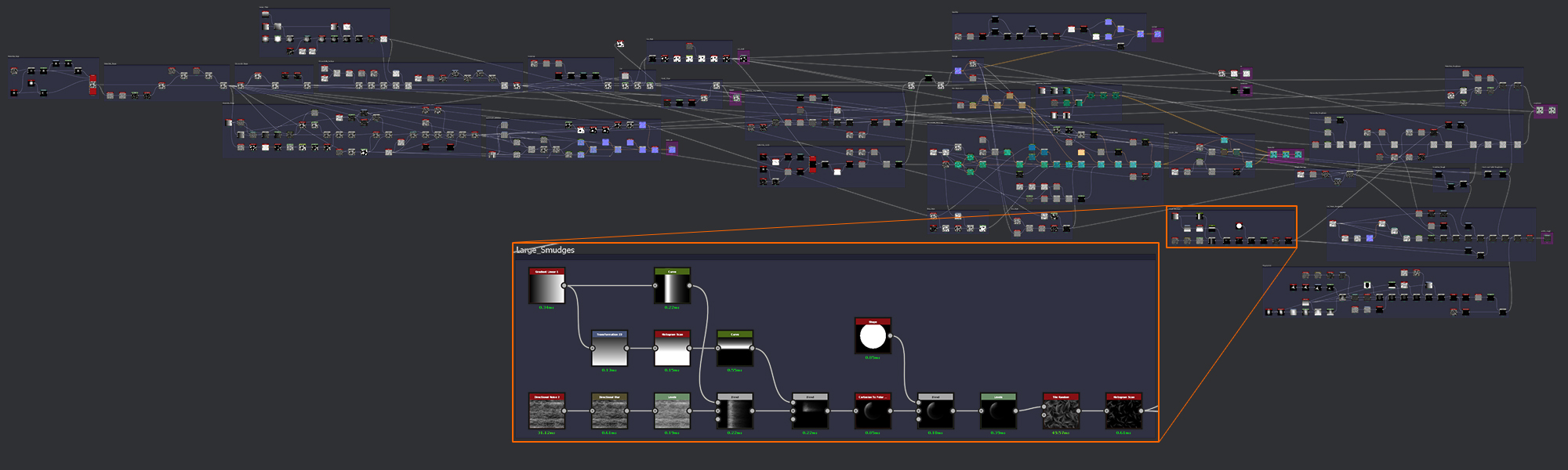
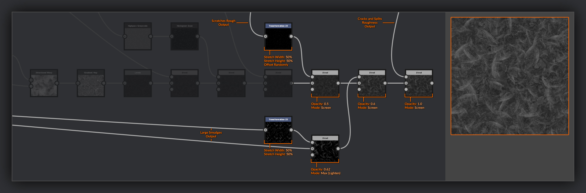
Large Smudges
Wanting more than these small smudges, I’m now going to create some even larger smudges to scatter around the surface of my Chrysocolla. As these will be another detail I’m sure to find useful later on, they too get the separate frame treatment.
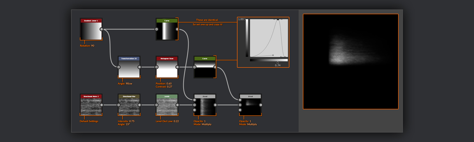
I start the smudges with a Directional Noise 2 to give some streaky noise. I put this through a Directional Blur node with a low intensity and a 15-degree angle to remove some of the sharpness from the directional noise. I then add a Levels node to bring the Levels Out Low up from black a bit.
The next step is to create some gradients to shape the smudge with. I start with a
Gradient Linear 1 with a 90-degree rotation. I feed this into a Curve node where I plot out a sweeping ridge shape. I combine this with my noise using a Blend node set to Multiply. This will take care of the shape of the smudge along the length. Next I’ll do a similar pass for the width. I start by rotating the Gradient Linear 1 from before 90 degrees clockwise in a Transform 2D node. I then pass this into a Histogram Scan node in which I adjust the contrast and position to shift the black to white range of the gradient. This will allow me to control the width of my smudges. Finally I copy my Curve node from before and hook this new rotated gradient into the input. I combine this with my noise using a Blend node set to Multiply as before.
I then put my linear smudge shape through a Cartesian to Polar Grayscale node to give it a radial swipe shape. To clear up the small amount of wrap-around in the corners I create a Shape node with the disc shape selected and drop the scale down slightly. I combine this disc with my smudge using a Blend node set to multiply to cut out everything outside the disc.
As a finishing touch to my smudge, I add a Levels node where I bring up the Levels in Mid slightly to shift the balance of my smudge towards the leading edge.
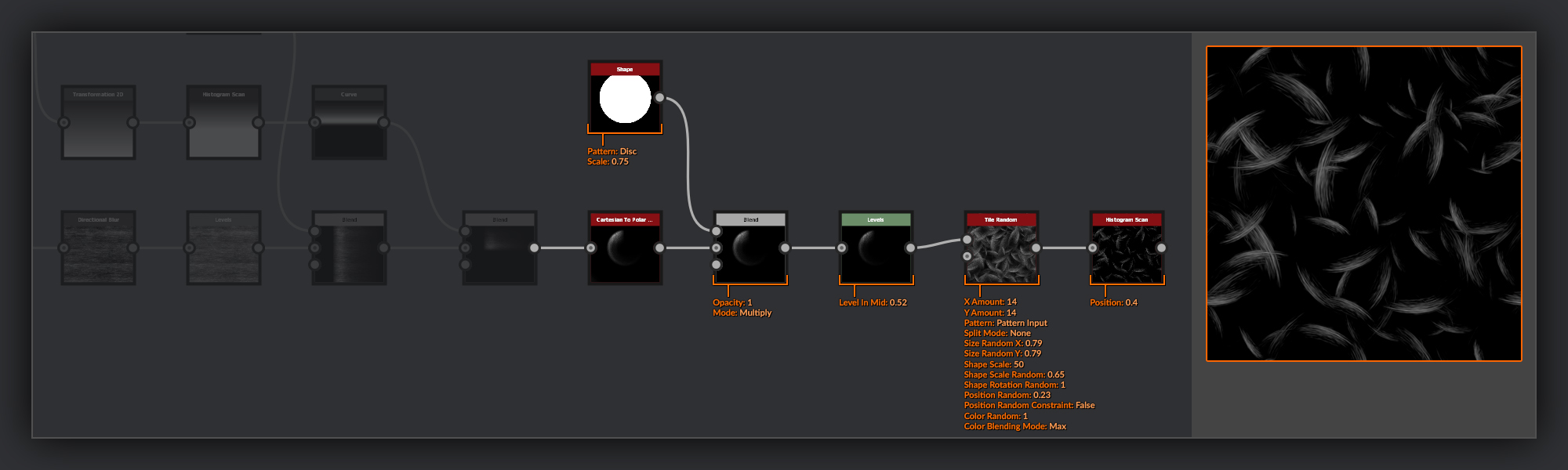
After finishing my smudge shape I scatter it across the canvas in a
Tile Random node with a mixture of scales, rotations and luminosities. Finally I add a Histogram Scan node to select just a few of the brightest parts of my smudges for combining with my roughness maps.
Back to Chrysocolla Roughness Again
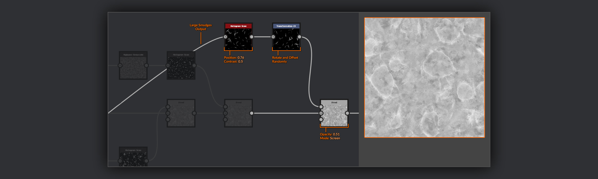
Back in the Chrysocolla Roughness I take the output of my large smudges and put it through another Histogram Scan node to further increase contrast and refine the selection. As I’m dealing with a rougher surface in the chrysocolla I want these smudges to have a slightly more aggressive shape, more like scrapes in the surface.
I then put this Histogram output through a Transform 2D to mix up its rotations from the base smudges. I don’t pay too much attention to how the smudges end up placed. I like to embrace the chaos in situations like this where it can help make a surface feel more organic - it can look odd if all the various details are too evenly distributed on a surface. I combine these refined scrapes with my Chrysocolla Roughness, using a Blend node set to Screen with a middle opacity.
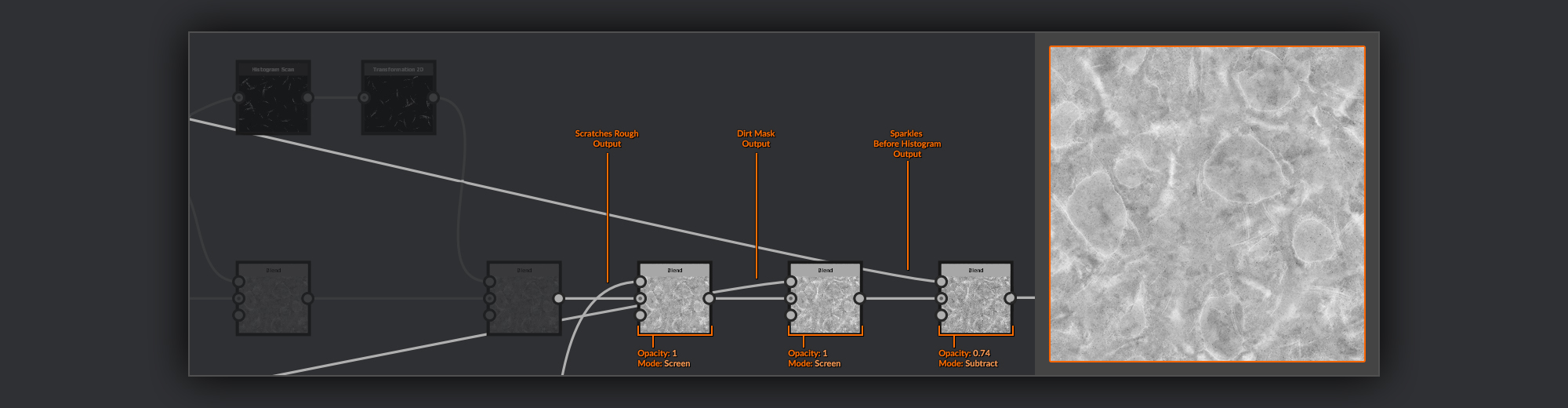
Scratches Rough
Next I’ll add the scratches from my Heightmap into the Roughness, as well as some extra scratches that will only be present in the Roughness. As I’ll use these in a couple of places I’ll create these in their own frame, separated from my Chrysocolla Roughness again.
From my scratches height frame I take the output of the Blend node used to add the noise into the scratches. I put this into a Transform 2D to again do some random placement for these extra scratches. I then put these transformed scratches into the input of a Directional Warp node
, I use the output of my Chrysocolla Surface in the Intensity Input. I adjust the Intensity and Warp Angle so the scratches conform to the Chrysocolla surface below them.
Finally I combine the output of this directional warp with the output of the directional warp in my scratches frame using a Blend node set to Max (Lighten).
Back to Chrysocolla Roughness for Finishing
Back in the main Chrysocolla Roughness string I add the scratches to my Chrysocolla Roughness using a Blend node set to Screen.
After the scratches the last couple of bits I want to add are going to be pulled from the masks I made previously in the BaseColor.
First I take the dirt mask I made in the Basecolor pass and add this to my Chrysocolla Roughness using a Blend node set to Screen. Next I take the mask for the Sparkles from just before I put it through the Histogram Scan. I combine this with my Chrysocolla Roughness in a Blend node set to Subtract; this will give each sparkle some glossiness to ensure they glint in the light.
And that is it for the Chrysocolla Roughness. I’ll frame it up to keep it all tidy.
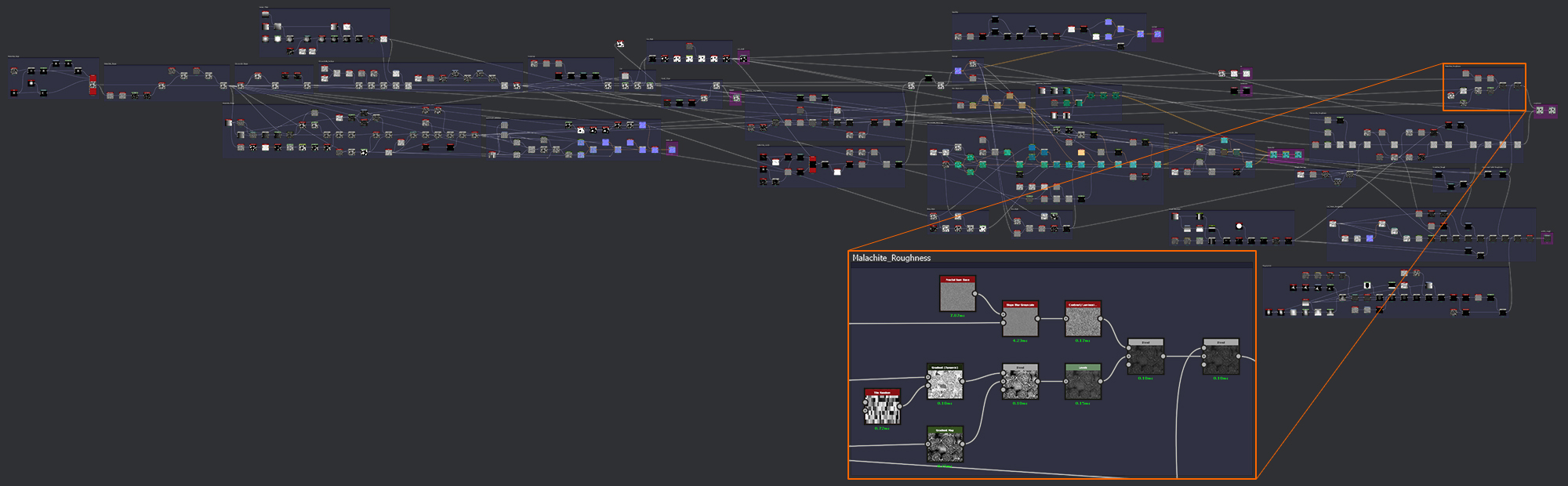
Malachite Roughness
Next we’ll do a similar treatment for the Cut Malachite faces.
I start by taking the auto-levelled output of my malachite rings frame. I put this into a Gradient Map node where I mix the black and white values up slightly. I don’t want the roughness variation to match up perfectly with the color variation. This will help add in that extra layer of interest separate to the color. I often try not to double up on these subtle layers of information between BaseColor and roughness in this way.
Next, as I have done many times before, I’ll create a palette - this, however, shall be the last! As in the Malachite Rings previously, I create a Tile Random node, again using the default square shape and with the Color Random variation up full. I use this palette in a Gradient (Dynamic) node Gradient Input, and the malachite rings frame output in the Grayscale Input. I then combine this output with that of my Gradient Map in a Blend node set to Overlay.
I put this malachite roughness into a Levels node and clamp my Levels out Min and Levels out Max to some darker grays, which will give the malachite a smoother glossy appearance.
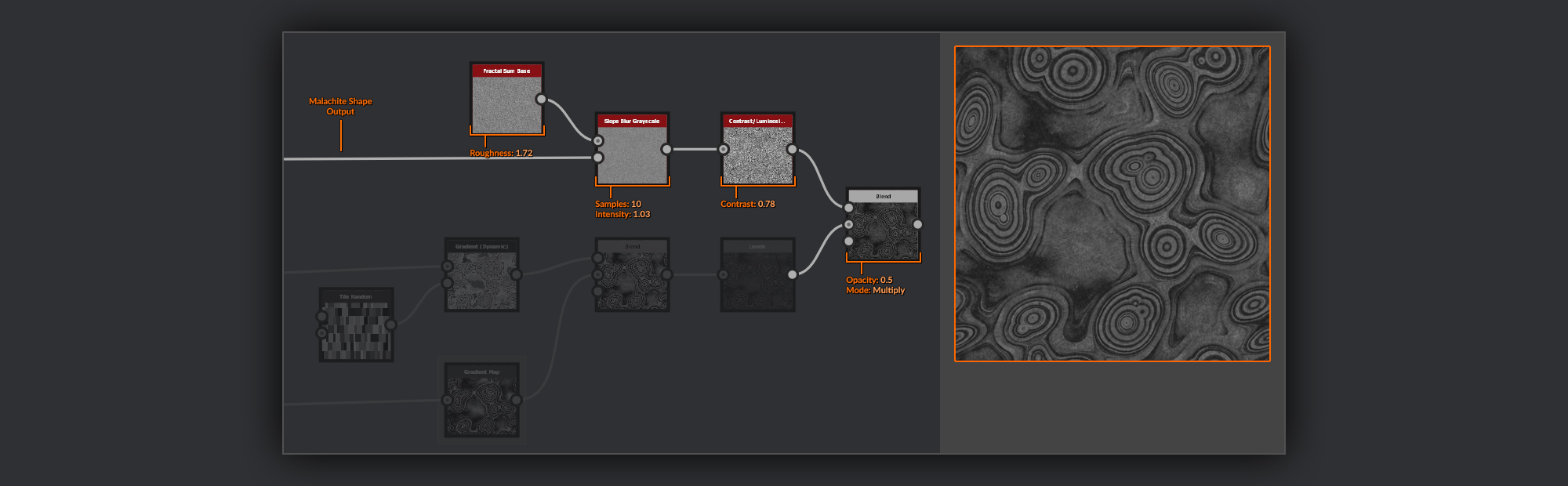
In the Mattershots reference you can see a slight crystalline growth pattern in the rings of the malachite. I want to add that to my material here.
To create that crystalline look I take a Fractal Sum Base node with its Roughness value increased. I pass this into the Grayscale Input of a Slope Blur Grayscale node; in the Slope input I use the output of my Malachite Shape frame. The Slope Blur then blurs the noise in a radial pattern around the peaks in the Malachite Shape Heightmap. I put the output of the Slope Blur grayscale into a Contrast/Luminosity node and bring up the contrast. Next I combine this with the rest of my Malachite Roughness string in a Blend node set to Multiply with a medium opacity.
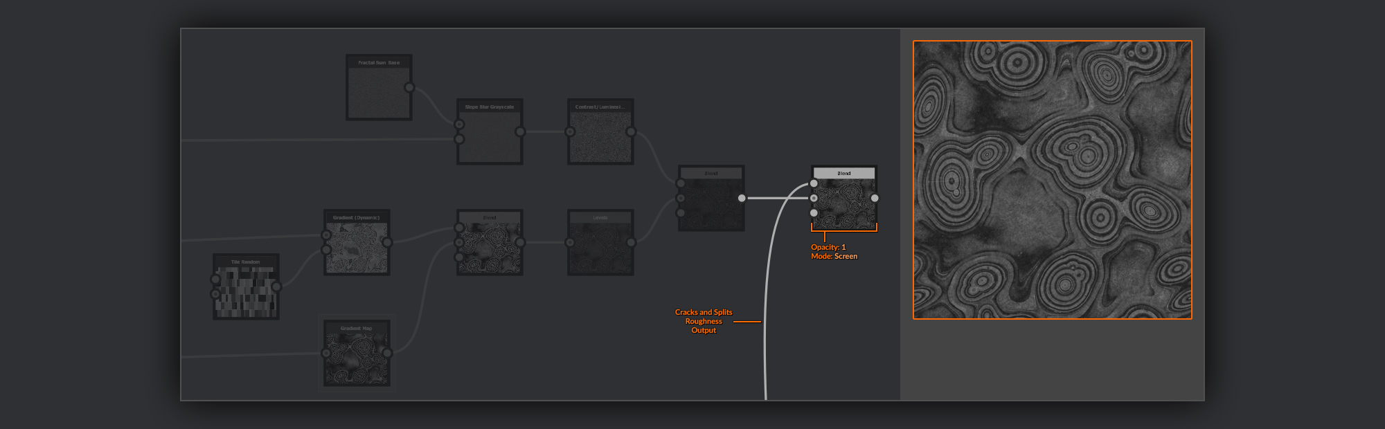
Cracks and Splits Roughness
The last thing I want to add in to my malachite Roughness is a combination of the cracks and splits from my malachite surface. I’ll put these in a separate frame again as I’ll want to reuse them in the polish roughness.
I take both the output of the splits frame and the cracks frame and combine them in a Blend node set to Max (Lighten)
. After this combination I Use a Levels node to lower the Levels In Max, brightening up my combined cracks and splits.
Back to Malachite Roughness
I add this in to my Malachite Roughness using a Blend node set to Screen.
Finishing Malachite and Chrysocolla Roughness
Finally, as with the BaseColor before, I need to combine the Malachite Roughness and the Chrysocolla Roughness.
I do this with a Blend node again and I use the Cut Mask from earlier in the opacity input to mask the two surfaces from each other. I then move my output node to the end of this chain.
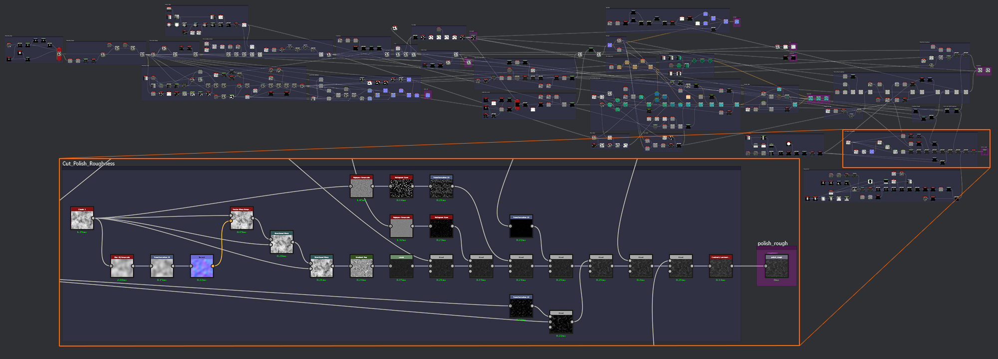
Cut Polish Roughness
As I mentioned at the beginning of this section on roughness, there are two Roughness maps I am going to need for my material. I’ve taken care of the Malachite and Chrysocolla Roughness, so all that’s left now is to create the Roughness for the cut surface polish.
This polish Roughness map will be a collection of noises and larger shapes to add some visual interest to the surface of the Malachite. I really want this piece to look like it’s been around for a while, so I’m not going to aim for a very clean polished surface.
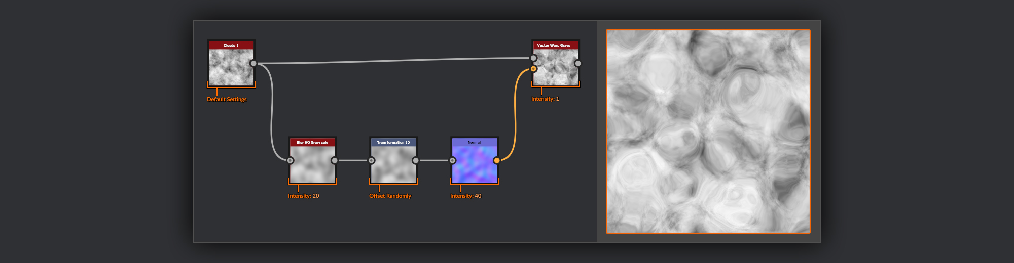
I’m going to start by making some streaky grayscale values as the base for my polish.
To begin my streaks I take a Clouds 2 node; I’ll put this through a Vector Warp Grayscale node to get some slight swirly patterns. To do this I need a Vector Map though, so I’ll make one from the Clouds 2. First I blur the clouds with a Blur HQ Grayscale node, I follow this with a Transform 2D node, applying a random transformation so my peaks don’t match up with the standard Clouds 2 input to the Vector Warp. Finally I’ll convert this to normal information in a Normal node. The output of this is put into the Vector Map input of the Vector Warp Grayscale.
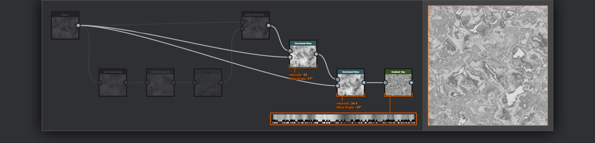
Next I’ll put the output of the Vector Warp Grayscale through a pair of
Directional Warp nodes to further break up the shapes. I use the unadjusted Clouds 2 as the Intensity input. I set the two warps to act in perpendicular directions to each other to break up any smooth lines in the warped noise.
Finally I put this through a Gradient map filled with some random grayscale points to generate some bands.
Before continuing I add a Levels node to bring the Levels High Out down and the Levels Low Out up slightly. I move these my levels range towards the lower end of the scale as I want the cut surface to be relatively glossy, but not a mirror finish.
The next few steps of the process involve mixing in the various shapes and noises I have created previously.
For the first pass I’ll focus on some patchy and dotty noises. I bring in the Rough Patches I created for the Chrysocolla Roughness, and add this into my Cut Polish Roughness using Blend node set to Max (Lighten). After this I go back to my small smudgy shapes in the Chrysocolla Roughness and grab the output of the Slope Blur Grayscale node. I put this into a Highpass Grayscale node with a small radius, I then use a Histogram Scan node to grab some small spots from this. I add these spots to the Cut Polish Roughness using a Blend Node set to Screen with a low opacity.
After these smaller spots I do a similar process again for some medium spots. I use the Clouds 2 from the beginning of my Roughness, and I repeat the chain of Highpass Grayscale to Histogram Scan nodes, and then I randomise its position slightly using a Transform 2D node. This is then added to the Cut Polish Roughness using a Blend node set to Screen with a very low opacity - I want to keep these medium blotches somewhat subtle.
In the second pass I’ll add in the various larger shapes I’ve created previously.
To begin I grab the combined scratches from the Chrysocolla Roughness, these I put through a
Transform 2D, reducing their scale by half and rotating and translating them a little. I add them to the Cut Polish Roughness using a Blend node set to screen with a medium opacity.
Next I take the output of my Large Smudges. I put an instance of this through a Transform 2D node where I halve its size. I then combine this with an unscaled copy in a Blend node set to Max (Lighten) with a medium opacity, so that these smaller smudges are less prominent.
Finally I’ll add in the Cracks and Splits Roughness from the surface of the cut Malachite using a Blend node set to Screen.
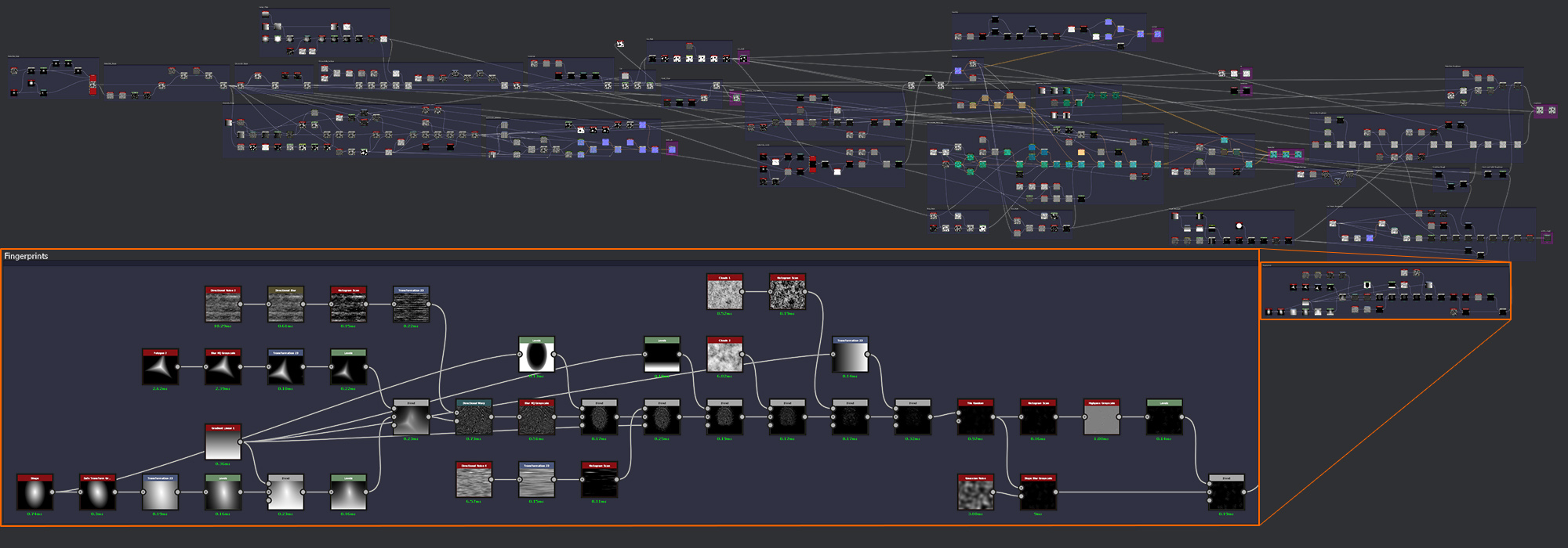
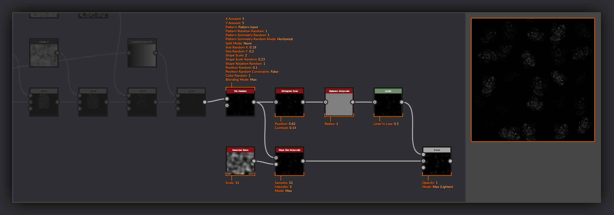
Fingerprints
At this stage I felt that overall my piece was missing something to give it a sense of scale. Although people may be familiar with the usual size of a cut mineral, I really wanted to add a feature that would sell this as a small sample, as the one in the Mattershots reference appeared to me.
The idea to help sell scale that I came up with, is to add fingerprints to the roughness of this polish layer. They will hopefully help to add a sense of scale quite naturally as fingerprints all usually fall within a pretty standard range of sizes. As well as adding a point of reference for scale, they will also help contribute to the handled look, hopefully boosting the realism and adding some sense of history to the piece.
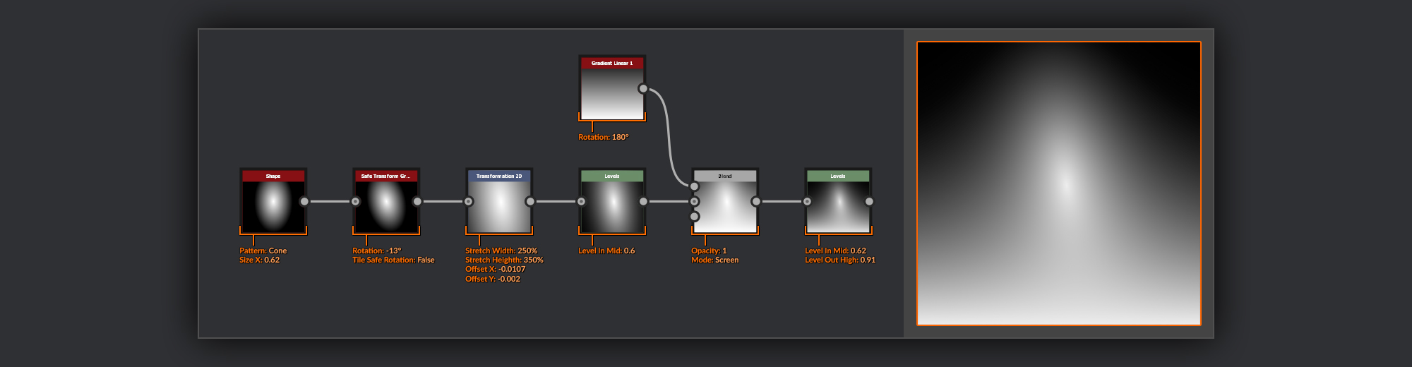
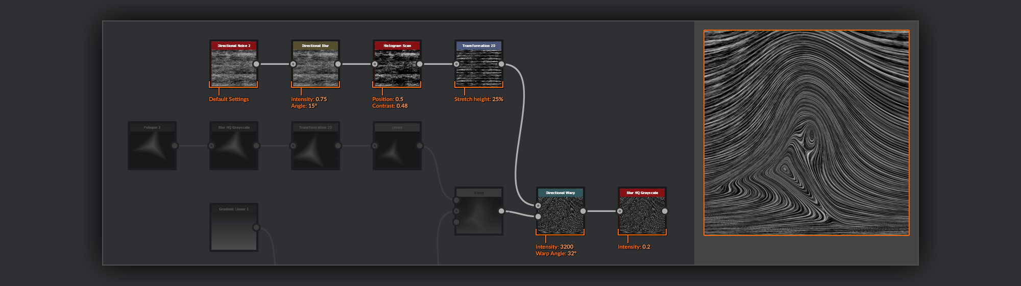
To create my fingerprint shape I’ll warp some banded noise over a collection of shapes often present in fingerprints.
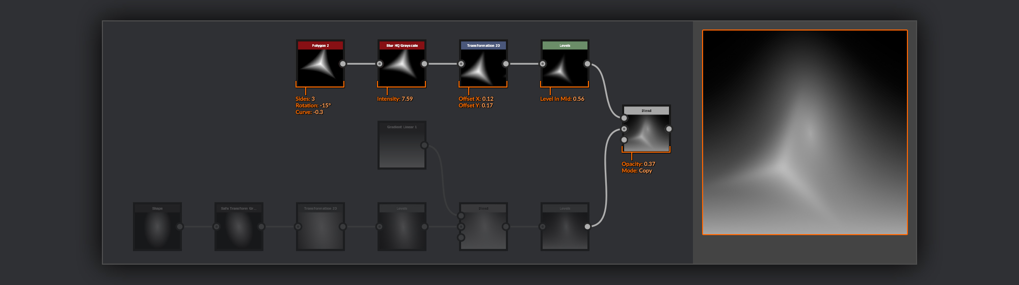
The obvious place to start is with a rough fingertip shape. For this I’m going to choose a Shape node with its pattern set to Cone, and I’ll reduce the width to make it slightly more slender, like a fingertip.
Next, I turn the shape into the beginning of the scaffold I’ll use to warp my noise later.
I first rotate the shape using a Safe Transform Grayscale node before scaling it further in a Transform 2D
node by 250 width and 350 height. I often like to split stages of a transformation process up between nodes like this, especially when I want more control over the exact placement and scale of an item after rotating or scaling. having the two nodes means I can, for example, make changes to the transformation independent of the rotation.
After this I use a Levels node to bring the Levels In Mid up, as this helps accentuate the shape towards the tip of the cone. This will give me tighter bands towards the center of my fingerprint. Then I create a Gradient Linear 1 node and add this into my fingerprint scaffold using a Blend node set to Screen. This will mean that the noises should flatten out towards the bottom of the fingerprint as they do in your average fingerprint. After this I add another Levels node
to bring the Levels In Mid up again, further accentuating the curve in the gradient between the highs and lows.
Most fingerprints are made up of a few recurring shapes. It’s the arrangement of these shapes and the number of bands around them that make your personal fingerprint unique. Generally people only have one or two shapes on each fingerprint, but it is possible for you to have more. Right now I’ll end up with a rather plain Whorl fingerprint, a single shape, so I’m going add another shape to make it more interesting. Specifically a shape known as a Tented Arch.
To start my arch I use a Polygon 2 node
set to 3 sides, I add a slight rotation here and also add a negative value to the curve to reduce the geometric shape slightly. After this I soften the shape with a Blur HQ Grayscale. This is to ensure the fingerprint doesn't end up with very sharp corners. I then add a Transform 2D node with which to adjust the shapes’ placement on the fingertip. I’ll make my final position adjustment once this shape has been blended into the fingerprint scaffold and I’m able to properly see my result.
Before I combine this with my fingerprint scaffold I add a Levels node to repeat the process of bringing the Levels In Mid up for this shape. Finally I combine this with my fingerprint scaffold below using a Blend node
set to Copy and a below mid opacity. At this point you can also make some tweaks to the position of the various shapes as you can now see how they all fit together.
With the scaffold complete I can move on to creating the ridges that will flow around the shapes I have set up in my fingerprint scaffold.
For the noise to make the ridges of my fingerprint I create a Directional Noise 2, then I pass this through a Directional Blur node to remove some of the finer details in the noise. I use a Histogram Scan node to increase the contrast and adjust the balance between highs and lows, before finally putting it through a
Transform 2D node to reduce the vertical height to 25%; this will increase the number of horizontal bands.
Now it’s time to turn this noise into an actual fingerprint. I add a Directional Warp node and use my fingerprint scaffold as the Intensity input. To push my ridges into a desired place I need to use an extremely high intensity and a direction perpendicular to my noise. The result from the Directional Warp is extremely noisy so I use a Blur HG Grayscale node to reduce this by blurring it with a small radius.
With my ridges defined it is now time to refine them a little to create the shape of an actual fingerprint.
I do this by taking the oval shape I started with and putting it into a Levels node. Inside the Levels node I bring the Levels In Low up slightly just to reduce the overall size. Next I bring the Levels in High down significantly to increase the flat surface on top of the shape and reduce the Levels In Mid to shift the falloff to give the shape a slight bulge. Finally I flip the Levels out Low and the Levels out High to invert them. I use this in the foreground of a Blend node set to Subtract to remove all the ridges from the outside of the fingerprint.
Even fingerprints have some fold lines in them - these are not only found around the knuckles. So I’ll add them into my recreation here.
For this, I take a Directional Noise 4 and stretch it in a
Transform 2D node, before using a Histogram Scan node to select a few of the highest ridges. I then remove these ridges from my fingerprint using a Blend node set to Subtract.
Finally, as most fingerprints left on a surface are not perfectly round I’ll flatten the bottom of the print slightly where the finger loses contact with the surface. I add a Levels node with the Gradient 1 from before as its input, I use this to clamp the gradients Highs and Lows to a bar across the bottom, and I then remove this from the fingerprint using another Blend node set to Subtract.
Now it is time to add add some imperfections to the fingerprint with a couple of noises.
First up I add a Clouds 2 and then combine this with the fingerprint in a Blend node set to Multiply. After this I’ll add some finer, more contrasting noise with a Clouds 1 and a Histogram Scan to select just some of the high points. I remove this noise from my fingerprint using a Blend node set to Subtract and a low opacity, so as to not completely remove my ridges in any spot. Finally I take the linear gradient from earlier and put it through a Transform 2D to rotate it by 90 degrees. I then multiply this over my fingerprint in a Blend node to give the look of an uneven pressure on the surface.
The fingerprint itself is now finished so I scatter the fingerprints across the surface of malachite using a Tile Random, with randomised Symmetry, Scale and Colour Random to mix up their appearance.
The last simple modifications I make to my fingerprints are to add some smudging with a Slope Blur grayscale; I use a Gaussian Noise in the slope input to provide a random direction and set the mode to Max. Then, to sharpen up the fingerprints and bring some detail back into the ridges, I take the output of the Tile Random and put it through a Histogram Scan node
to select just the highest parts of the fingerprint ridges. Next I put the output through a Highpass Grayscale node with a low radius, and a Levels node with the Levels in Low brought up to the mid-point, cutting out anything but the tops of the ridges. Finally I combine this with the smudged version in a Blend node set to Max (Lighten)
Back to Cut Polish Roughness
The last things to do for the Cut Polish Roughness is to add in my fingerprints which I do in a Blend node set to Screen with a middle opacity. I also add a Contrast/Luminosity node where I can use the luminosity to quickly adjust the how glossy the surface of my polish will be.
Finally I frame up all the nodes needed for Cut Polish Roughness, and hook it up to its own output node.
Making the MDL
Now that I have the Substance graph finished, it’s time to move on to constructing the MDL graph that I’ll use to define the exact surface properties of my piece.
To add an MDL graph, right click on your Package in the Explorer panel and choose MDL Material from the new menu. From the New MDL Graph window I choose to use the Dielectric Graph Template as the base of my MDL. It features the nodes I need to set up the Chrysocolla surface, which is the more simple of the two surfaces my piece is composed of. On top of this template I’ll then add the extra nodes that will be needed to render the Cut Malachite surfaces and their polished clear coat layer.
With the new MDL graph now set up I begin by bringing in the Substance graph, simply dragging and dropping it in from the Explorer to the graph. Once it’s available I’ll make sure the Output Size is set where I want it. For the materialize contest the required output resolution was 4096 x 4096, so I’ll set my graph to that in the SBS Base Parameters.
Chrysocolla MDL
Now with the pieces in place it’s time to start building up our MDL. I’ll begin with the section that is going to handle the appearance of the Chrysocolla, which is the most simple of the two surfaces to set up, as most of the nodes I’ll use are already present in the template I have chosen.
I’ll start by plugging in the outputs of my Substance graph in to the appropriate inputs for the MDL. I plug in the BaseColor, Normal and Roughness. The BaseColor and Roughness can both be connected straight to their respective inputs. The Normal map needs to be added in place of the Normal node that is present in the default MDL. For now, these are the only outputs of my graph that I have the option of using in my MDL, so I’ll need to add new nodes for each subsequent piece.
The first new section I am going to create will allow me to utilise the Heightmap from the Substance Graph as a Heightmap for tessellation in the MDL. I create a Displacement node
for the height input, and I use the Heightmap output of the Substance graph. In the heightScale input I create a Float node. This will contain the value that will be used in the MDL to control the intensity of the displacement effect. I then connect the output of this Displacement node to the corresponding input of the Material Geometry node.
The next section I’ll add will layer in the ambient occlusion pass on top of the material. For this I start with a Weighted Layer node which I add between the custom Curve Layer node and the Material Surface node, before it reaches the material output. I connect it using the layer input. In the base input I create a new Diffuse Reflection BSDF node
and set its tint (color) to black, and put it’s roughness up full to represent the darkness in the recesses of the Chrysocolla surface. Finally I use the AO output of my Substance Graph as the weight input so that the full Chrysocolla surface shows through where the AO mask is white, while the blackened base BSDF is confined to the darker areas of the AO mask.
MDL Malachite Anisotropy
Now that I’ve taken care of the more straightforward Chrysocolla surface I’ll add the sections that are going to deal with the surface of the Cut Malachite. I’m going to add two passes for the Malachite, a layer of Anisotropic reflection to mimic the way the light scatters over the crystalline structures visible in the Mattershots reference that will make use of the anisotropic direction map I created, and the layer of polish on the surface for which we previously created the Roughness. I’ll start with the Anisotropy.
I’ll start with an Anisotropy Conversion node
which will process the information necessary for generating the anisotropic highlights. I connect the multiplied Roughness output to the Roughness input, and my anisotropic direction map output to the tangent_u input. I then create 2 Float nodes. I connect the first Float node to the anisotropy input; the second node I connect to the anisotropy_rotation input.
To turn the output of the Anisotropy Conversion node into renderable information I’ll connect the output to a Microfacet GGX Smith BSDF node. For the tint input I’ll add an Operator+ node; in the y input I use the BaseColor output of my Substance Graph. In the x input I add a Color node
and set the color to a slightly brighter shade of the average green in my malachite. This will help make the highlights in the anisotropic reflections stand out from the background malachite.
The final step in my Anisotropic pass is to blend it in to the Chrysocolla BSDF. I add a Weighted Layer node. I feed the Chrysocolla output in to the base input, and place the output of my anisotropy in to the layer input. In the weight input I add a Float node which I will use to control the strength of the anisotropic highlight over the regular surface.
MDL Malachite Polish
After the Anisotropy the final piece to add to my MDL is a pass to do the layer of polish over the surface of the Cut Malachite.
I start by taking the polish_rough output from my Substance graph and, as in the template I started with, I’ll square it by passing it through an Operator node in both the x and y inputs. Then in a Microfacet GGX Smith BSDF node
I use this squared Roughness for both the roughness_u and roughness_v inputs.
To make this look like a layer of polish over the malachite beneath I need to add it as an extra layer of reflection information.
To do this I’ll create a Fresnel Layer node and use the output of the malachite layer in the base input; in the layer input I add my polish. Now I’ll need to define the index of refraction for my polish. I add a Float node to hold the value and hook it up to the ior input of the Fresnel Layer node. Clear polish has a value around 1.5, but I ended up pushing it slightly higher than that when tweaking for purely artistic reasons.
The final step needed to complete the MDL Graph is to combine this polished Malachite with the Chrysocolla. I’ll add another Weighted Layer node. I put my Chrysocolla output in the base and add my Cut Malachite in the layer input. Finally, take the cut_mask output of my Substance graph and use that in the weight input so that the two surfaces are separated correctly.
Final Renders
The very last piece of the puzzle to cover is the set up I used for the final renders in my submission to the Materialize competition. Before beginning my render setup I did a couple of small tweaks to my material. In the MDL I chose to push the Displacement up even further. I ended up doubling the scale value to 8, I also set the material to tile 1.25 times inside the malachite_with_chrysocolla_tutorial Substance node parameters. And I also chose the Plane (hi-res) geometry from the Scene menu of the 3D View.
Now that I’m ready to render, the first thing I do is set Use Window Resolution
to false in the camera settings panel. I also set the resolution at which I want to output my image. This means the 3D window is now going to give me a preview of the framing I’ll have in the final output by letterboxing either the top or bottom of the view if its dimensions don’t already match the ratio of the Camera Resolution I’ve chosen. This is going to be a lot more useful to me while I set up the shot I want.
Before I start positioning my camera, I usually lower the Max Samples in the renderer settings panel. I normally use a relatively low number, like 20, just to speed up the process slightly. While positioning my camera I also adjust the Focal Length (mm) position to find a result I like.
At the same time as I’m working out the camera placement I play with the rotation of the 3D View Environment
to get some interesting light-play across the surface of my piece. For my renders I used the corsica_beach Environment.
Once I’ve got the camera positioned nicely I adjust the Focus Distance and Aperture Diameter to get some subtle depth of field going. I don’t want to overdo the effect, I like to use just a small amount to persuade the viewer to focus on the detail I’ve picked out in my render.
With the camera set up as I like it I start tweaking the Post Effects Options. In this case I didn’t do anything very special. I tried to build the material in a way that I could rely on to provide the visual response I wanted on its own. All I did in the camera settings was to massage the result ever so slightly with a small amount of post-processing adjustments.
I tweaked the glare settings to make them a little more subtle. I like to keep some of the glare present as it slightly softens the harshness of the strong highlights on the polished surfaces. I put the Quality setting down to blur the Glare shapes slightly. I also Increased the Threshold so the bursts of Glare only appear strongly in the brightest spots. Lastly I chose Bloom as the Shape, as it doesn’t have as many of the lens flare type artifacts as the other shapes.
I increased the Vignette Strength to enhance the close up, and give a macro-style feeling of the shot.
Under Colour Correction I ever so slightly increased the contrast so the range of brightnesses felt a little more dynamic. This also helps the detail in the material to pop a little better, especially in the Cut Malachite faces.
Finally, in the Tone Mapping I slightly increased Exposure and Gamma to brighten up the image a little. I also chose Sensitometric as the Tone Mapping Function.
And here’s a shot of my render with the post effects applied.
Outro
That’s it! We’ve everything that went into making this piece, from blank canvas, to final renders. I hope you’ve found this useful - and congratulations if you made it all the way through. If you’ve just skipped to the end searching for enlightenment, then I’m afraid you’ve missed all the good bits in the middle.
You can control how Adobe websites use cookies and similar technologies by making choices below. But note that if you disable cookies and similar technologies entirely, Adobe websites may not function properly.
Cookies are small text files stored by your web browser when you use websites. There are also other technologies that can be used for similar purposes like HTML5 Local Storage and local shared objects, web beacons, and embedded scripts. These technologies help us do things like remembering you and your preferences when you return to our sites, measure how you use the website, conduct market research, and gather information about the ads you see and interact with.
You can make choices in the menu below about what cookies and other technologies you want us to use on Adobe sites when you visit them from this browser. You can always change those choices later by clicking on the Cookie Preferences link at the bottom of the page.
If enabled:
We can improve your experience by tailoring the site and the content to things we think might be of interest
We can better keep track of your preferences — like what language you prefer to use
We will better understand your likely interests so we can provide you more relevant Adobe ads and content on non-Adobe websites and in non-Adobe apps
It will help us improve the performance of our website and those of our partners who use the Adobe Experience Cloud
If disabled:
We won’t be able to remember you from session to session so the experience may not be tailored to your interests
You’ll still have access to the content of the site but certain features that depend on cookies may not function
You’ll still see ads, they just may not be as relevant to you
General information
You can control how Adobe websites use cookies and similar technologies by making choices below. But note that if you disable cookies and similar technologies entirely, Adobe websites may not function properly.
Cookies are small text files stored by your web browser when you use websites. There are also other technologies that can be used for similar purposes like HTML5 Local Storage, web beacons, and embedded scripts. These technologies help us do things like remembering you and your preferences when you return to our sites, measure how you use the website, conduct market research, and gather information about the ads you see and interact with.
You can make choices in the menu below about what cookies and other technologies you want us to use on Adobe sites when you visit them from this browser. You can always change those choices later by clicking on the Cookie Preferences link at the bottom of the page.
If enabled:
We can improve your experience by tailoring the site and the content to things we think might be of interest
We can better keep track of your preferences — like what language you prefer to use
We will better understand your likely interests so we can provide you more relevant Adobe ads and content on non-Adobe websites and in non-Adobe apps
It will help us improve the performance of our website and those of our partners who use the Adobe Experience Cloud
If disabled:
We won’t be able to remember you from session to session so the experience may not be tailored to your interests
We’ll still count your use of our site and services
You’ll still have access to the content of the site but certain features that depend on cookies may not function
You’ll still see ads, they just may not be as relevant to you
Operate the site and core servicesOperate site and measure engagement
Always active
These cookies are required, and they are used to enable the site and related services core functionality. Without them the site could not operate, so they cannot be disabled.
These cookies enable the site and related services’ core functionality and collect statistics about user engagement, such as counting active use to help us understand trends. These cookies cannot be disabled.
Measure performance
These cookies are used to analyze site usage to measure and improve performance. Without them Adobe cannot know what content is most valued and how often unique visitors return to the site, making it hard to improve information we offer to you.
These cookies are used to analyze site usage to measure and improve performance. Without them Adobe cannot know what content is most valued, making it hard to improve information we offer to you.
Extend functionality
These cookies are used to enhance the functionality of Adobe sites such as remembering your settings and preferences to deliver a personalized experience; for example, your username, your repeated visits, preferred language, your country, or any other saved preference.
Personalize advertising
These cookies are used to enable Adobe and our partners to serve ads more relevant to your interests. Without them you will still see ads, but they might not be as relevant to you.
Personalize advertising
These cookies are used to enable Adobe and our partners to serve ads more relevant to your interests. Without them you will still see ads, but they might not be as relevant to you.